9 Strip Plot Design
9.1 Background
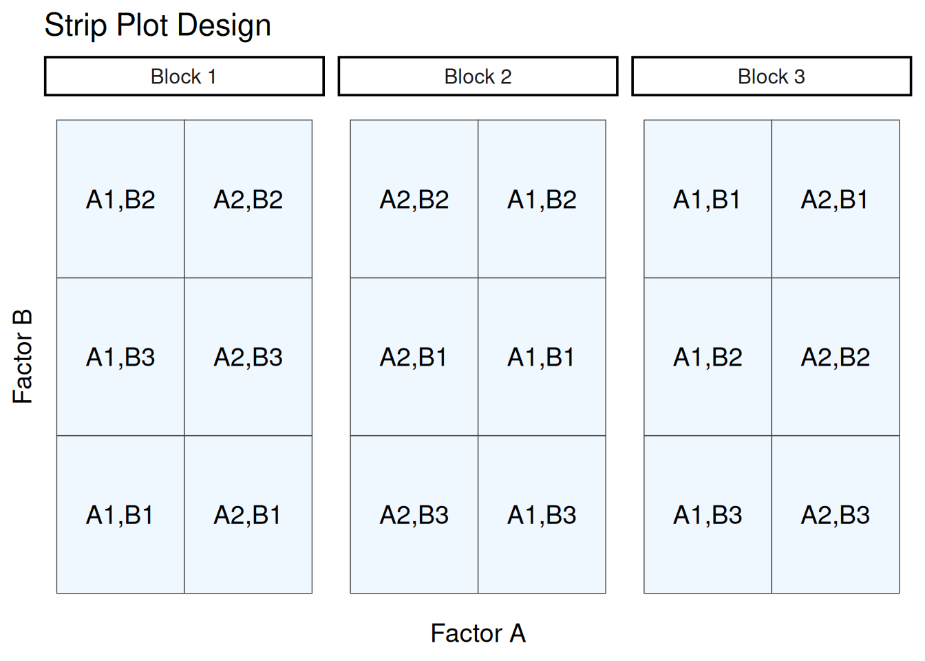
Also referred by “split block design”, this design can be very useful for agricultural field experiments when there are two treatments that need to be applied at a larger scale than the experimental units. It is a row-column design where treatments are applied in strips within each block. Below is an example layout of this design.
The statistical model for this design is:
\[y_{ijk} = \mu + \tau_i + \alpha_j + (\tau\alpha)_{ij} + \beta_k + (\tau\beta)_{ik} + (\alpha\beta)_{jk} + \epsilon_{ijk}\]
Where:
\(\mu\)= overall experimental mean, \((\tau\alpha)_{ij}\), \((\tau\beta)_{ik}\), and \(\epsilon_{ijk}\) are the errors used to test factor A, B, and their interaction AB, respectively. \(\alpha\) and \(\beta\) are the main effects applied A and B, and \(\alpha_j\beta_k\) represents the interaction between main factors.
\[ \epsilon_{ijk} \sim N(0, \sigma^2)\]
9.2 Example Analysis
We will start the analysis first by loading the required libraries for this analysis for lmer() and lme() models.
library(lme4); library(lmerTest); library(emmeans)
library(dplyr); library(performance); library(desplot)
library(broom.mixed)library(nlme); library(performance); library(emmeans)
library(dplyr); library(desplot); library(broom.mixed)
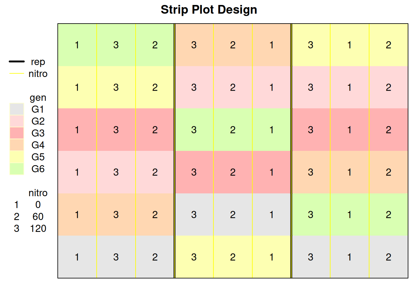
library(pbkrtest)For this example, we will use a rice strip-plot experiment data from the agridat package, “gomez.stripplot”. This data contains a strip-plot experiment with three reps, variety as the whole plot and nitrogen fertilizer as the whole plot applied in the strips.
rice <- read.csv(here::here("data", "rice_stripplot.csv"))| rep | replication unit |
| nitro | nitrogen fertilizer in kg/ha |
| gen | rice variety |
| row | row (represents gen) |
| col | column (represents nitro) |
| yield | grain yield in kg/ha |
The plot below shows the application of treatments in horizontal and vertical directions within a block in a strip plot design.
9.2.1 Data integrity checks
- Check structure of the data
The ‘rep’, ‘nitro’, and ‘gen’ variables in the data needs to be a factor/character variables and ‘yield’ should be numeric.
str(rice)'data.frame': 54 obs. of 6 variables:
$ yield: int 2373 4076 7254 4007 5630 7053 2620 4676 7666 2726 ...
$ rep : chr "R1" "R1" "R1" "R1" ...
$ nitro: int 0 60 120 0 60 120 0 60 120 0 ...
$ gen : chr "G1" "G1" "G1" "G2" ...
$ col : int 1 3 2 1 3 2 1 3 2 1 ...
$ row : int 1 1 1 3 3 3 4 4 4 2 ...Let’s convert ‘nitro’ from numeric to factor.
rice$nitro <- as.factor(rice$nitro)- Inspect the independent variables
Let’s running a a cross tabulation of independent variables to look at the balance of treatment factors.
table(rice$gen, rice$nitro)
     0 60 120
  G1 3  3   3
  G2 3  3   3
  G3 3  3   3
  G4 3  3   3
  G5 3  3   3
  G6 3  3   3
It looks balanced with 3 number of observations for each variety and nitrogen level.
- Check the extent of missing data
Next step is to identify if there are any missing observations in the data set.
colSums(is.na(rice))yield rep nitro gen col row
0 0 0 0 0 0 We don’t have any missing values in this data set.
- Inspect the dependent variable
Let’s check the distribution of dependent variable by plotting a histogram.
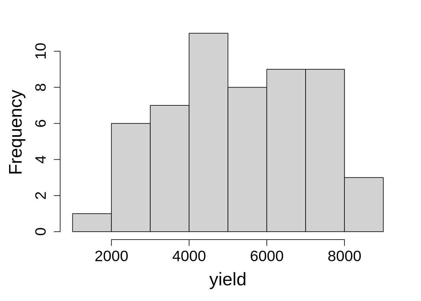
No extreme values or skewness is present in the yield values.
9.2.2 Model Building
The goal of this analysis is to evaluate the impact of nitrogen, genotype, and their interaction on rice yield. The variables “rep”, “gen” (nested in rep), and “nitro” (nested in rep) were random effects in the model.
model_lmer <- lmer(yield ~  nitro*gen +  (1|rep) +
                   (1|rep:gen) + (1|rep:nitro),
                   data = rice)
tidy(model_lmer)
# A tibble: 22 × 8
effect group term estimate std.error statistic df p.value
<chr> <chr> <chr> <dbl> <dbl> <dbl> <dbl> <dbl>
1 fixed <NA> (Intercept) 3572. 572. 6.24 17.8 0.00000732
2 fixed <NA> nitro60 1560. 558. 2.80 22.4 0.0104
3 fixed <NA> nitro120 3976. 558. 7.13 22.4 0.000000341
4 fixed <NA> genG2 1363. 717. 1.90 20.9 0.0714
5 fixed <NA> genG3 678. 717. 0.945 20.9 0.355
6 fixed <NA> genG4 487. 717. 0.679 20.9 0.504
7 fixed <NA> genG5 530. 717. 0.739 20.9 0.468
8 fixed <NA> genG6 -364. 717. -0.508 20.9 0.617
9 fixed <NA> nitro60:genG2 219. 741. 0.296 20.0 0.771
10 fixed <NA> nitro120:genG2 -1699. 741. -2.29 20.0 0.0328
# ℹ 12 more rowsrice$one <- factor(1)
model_lme <-lme(yield ~ nitro*gen,
random = list(one = pdBlocked(list(
pdIdent(~ 0 + rep),
pdIdent(~ 0 + rep:gen),
pdIdent(~ 0 + rep:nitro)))),
data = rice)
model_lmeLinear mixed-effects model fit by REML
Data: rice
Log-restricted-likelihood: -303.7102
Fixed: yield ~ nitro * gen
(Intercept) nitro60 nitro120 genG2 genG3
3571.66667 1560.33333 3976.33333 1362.66667 678.00000
genG4 genG5 genG6 nitro60:genG2 nitro120:genG2
487.33333 530.00000 -364.33333 219.00000 -1699.33333
nitro60:genG3 nitro120:genG3 nitro60:genG4 nitro120:genG4 nitro60:genG5
312.33333 -357.66667 -65.66667 -941.00000 -28.66667
nitro120:genG5 nitro60:genG6 nitro120:genG6
-2066.00000 -1053.33333 -4691.66667
Random effects:
Composite Structure: Blocked
Block 1: repR1, repR2, repR3
Formula: ~0 + rep | one
Structure: Multiple of an Identity
repR1 repR2 repR3
StdDev: 393.4278 393.4278 393.4278
Block 2: repR1:genG1, repR2:genG1, repR3:genG1, repR1:genG2, repR2:genG2, repR3:genG2, repR1:genG3, repR2:genG3, repR3:genG3, repR1:genG4, repR2:genG4, repR3:genG4, repR1:genG5, repR2:genG5, repR3:genG5, repR1:genG6, repR2:genG6, repR3:genG6
Formula: ~0 + rep:gen | one
Structure: Multiple of an Identity
repR1:genG1 repR2:genG1 repR3:genG1 repR1:genG2 repR2:genG2 repR3:genG2
StdDev: 600.1711 600.1711 600.1711 600.1711 600.1711 600.1711
repR1:genG3 repR2:genG3 repR3:genG3 repR1:genG4 repR2:genG4 repR3:genG4
StdDev: 600.1711 600.1711 600.1711 600.1711 600.1711 600.1711
repR1:genG5 repR2:genG5 repR3:genG5 repR1:genG6 repR2:genG6 repR3:genG6
StdDev: 600.1711 600.1711 600.1711 600.1711 600.1711 600.1711
Block 3: repR1:nitro0, repR2:nitro0, repR3:nitro0, repR1:nitro60, repR2:nitro60, repR3:nitro60, repR1:nitro120, repR2:nitro120, repR3:nitro120
Formula: ~0 + rep:nitro | one
Structure: Multiple of an Identity
repR1:nitro0 repR2:nitro0 repR3:nitro0 repR1:nitro60 repR2:nitro60
StdDev: 235.2591 235.2591 235.2591 235.2591 235.2591
repR3:nitro60 repR1:nitro120 repR2:nitro120 repR3:nitro120 Residual
StdDev: 235.2591 235.2591 235.2591 235.2591 641.5963
Number of Observations: 54
Number of Groups: 1
NoteCrossed random effects
This type of variance-covariance structure in nlme::lme() is represented by a pdBlocked object with pdIdent elements. The pdBlocked class is for blocked diagonal matrices and pdIdent creates identity matrices for each of the factors listed.
9.2.3 Check Model Assumptions
Let’s evaluate the assumptions of linear mixed models by looking at the residuals and normality of error terms.
check_model(model_lmer, check = c('qq', 'linearity', 'reqq'), detrend = FALSE, alpha = 0)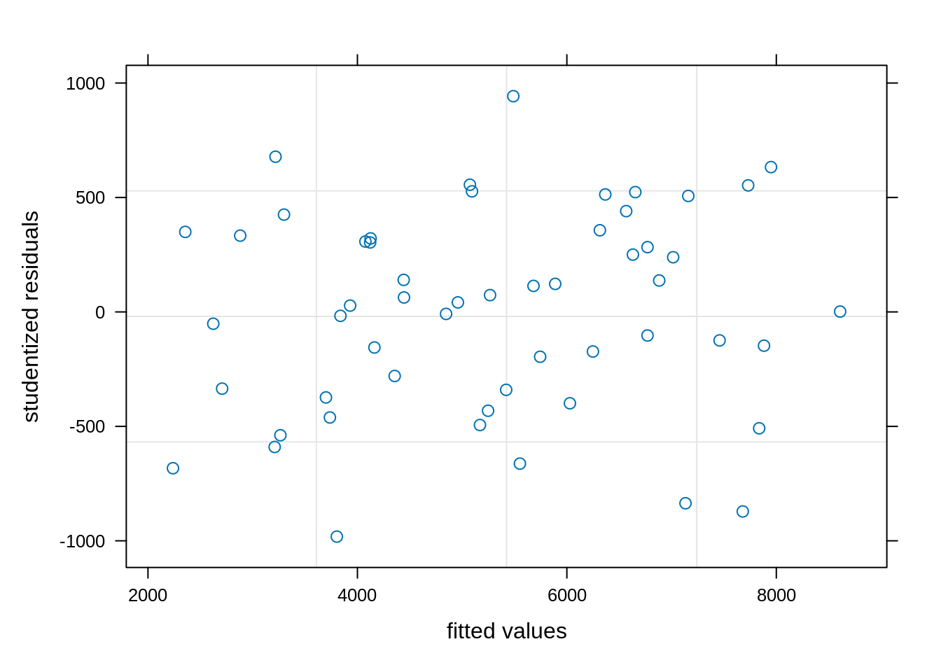
plot(model_lme, resid(., scaled=TRUE) ~ fitted(.), abline = 0,
     xlab = "fitted values", ylab = "studentized residuals")
qqnorm(residuals(model_lme)); qqline(residuals(model_lme))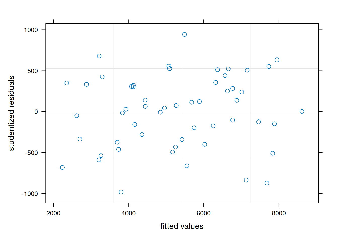
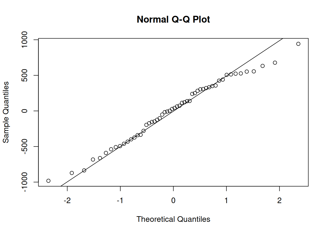
The residuals fit the assumptions of the model well.
9.2.4 Inference
We can evaluate the model for the analysis of variance, for main and interaction effects.
anova(model_lmer) Type III Analysis of Variance Table with Satterthwaite's method
Sum Sq Mean Sq NumDF DenDF F value Pr(>F)
nitro 28047925 14023963 2 3.9999 34.0682 0.0030751 **
gen 15751150 3150230 5 9.9999 7.6528 0.0033724 **
nitro:gen 23877979 2387798 10 20.0001 5.8006 0.0004271 ***
---
Signif. codes: 0 '***' 0.001 '**' 0.01 '*' 0.05 '.' 0.1 ' ' 1The anova() function for nlme does not handle the degree of freedom correctly for F-tests in the strip plot design, so we have to manually set it. This only works for balanced data. Wald chi-square tests can be conducted using car::Anova() and produce identical results for lme4::lmer() and nlme::lme().
rep_n = length(unique(rice$rep)) - 1
gen_n = length(unique(rice$gen)) - 1
nitro_n = length(unique(rice$nitro)) - 1
denominator_df = c(nitro_n*rep_n, gen_n*rep_n, nitro_n*gen_n*rep_n)

lme_aov <- anova(model_lme) |> as.data.frame() |>
  slice(-1) |> mutate(denDF = denominator_df) |>
  mutate(`p-value` = pf(`F-value`, numDF, denDF, lower.tail = FALSE))

lme_aov
numDF denDF F-value p-value
nitro 2 4 34.068996 0.0030746231
gen 5 10 7.652839 0.0033722261
nitro:gen 10 20 5.800612 0.0004270726Analysis of variance showed a significant interaction impact of gen and nitro on rice grain yield.
Next, We can estimate marginal means for nitro and gen interaction effects using the emmeans package.
emm1 <- emmeans(model_lmer, ~ nitro*gen)
emm1
nitro gen emmean SE df lower.CL upper.CL
0 G1 3572 572 17.8 2368 4775
60 G1 5132 572 17.8 3929 6335
120 G1 7548 572 17.8 6345 8751
0 G2 4934 572 17.8 3731 6138
60 G2 6714 572 17.8 5510 7917
120 G2 7211 572 17.8 6008 8415
0 G3 4250 572 17.8 3046 5453
60 G3 6122 572 17.8 4919 7326
120 G3 7868 572 17.8 6665 9072
0 G4 4059 572 17.8 2856 5262
60 G4 5554 572 17.8 4350 6757
120 G4 7094 572 17.8 5891 8298
0 G5 4102 572 17.8 2898 5305
60 G5 5633 572 17.8 4430 6837
120 G5 6012 572 17.8 4809 7215
0 G6 3207 572 17.8 2004 4411
60 G6 3714 572 17.8 2511 4918
120 G6 2492 572 17.8 1289 3695
Degrees-of-freedom method: kenward-roger
Confidence level used: 0.95 Nminus = length(unique(rice$rep)) * length(unique(rice$gen)) - 1
deg_free <- pbkrtest::get_Lb_ddf(model_lmer, c(1, rep(0, Nminus)))
emm2 <- emmeans(model_lme, ~ nitro*gen, df = deg_free)
emm2 nitro gen emmean SE df lower.CL upper.CL
0 G1 3572 572 17.8 2368 4775
60 G1 5132 572 17.8 3929 6335
120 G1 7548 572 17.8 6345 8751
0 G2 4934 572 17.8 3731 6138
60 G2 6714 572 17.8 5510 7917
120 G2 7211 572 17.8 6008 8415
0 G3 4250 572 17.8 3046 5453
60 G3 6122 572 17.8 4919 7326
120 G3 7868 572 17.8 6665 9072
0 G4 4059 572 17.8 2856 5262
60 G4 5554 572 17.8 4350 6757
120 G4 7094 572 17.8 5891 8298
0 G5 4102 572 17.8 2898 5305
60 G5 5633 572 17.8 4430 6837
120 G5 6012 572 17.8 4809 7215
0 G6 3207 572 17.8 2004 4411
60 G6 3714 572 17.8 2511 4918
120 G6 2492 572 17.8 1289 3695
Degrees-of-freedom method: user-specified
Confidence level used: 0.95 Without specifying the degrees of freedom, emmeans() is not able to estimate the confidence limits from this lme() model. In this case, the degrees of freedom are re-estimated from the merMod object.
Note
lme vs lmer
For strip plot experiment design, fitting nested and crossed random effects is more complicated to implement in nlme compared to lme4, and this complexity appears to complicate downstream estimation of the degrees of freedom. It is easier and statistically correct to use lme4, so understood if an analyst prefers this package for analyzing split plot experiments!
Sometimes, elements of split plot and split block are combined, resulting in strip-split plot design. Kevin Wright describes how to analyze this design in the ‘agridat’ package.