3 Mixed Model Background
3.1 Mixed model terms
Mixed-effects models are called “mixed” because they are modelling both fixed and random effects and estimating these effects jointly. These are also called “multilevel” or “hierarchical” models in reference to groups or clusters with a hierarchical structure where we expect the groups to have correlations between their groups members.
This tutorial concerns general linear mixed models (sometimes abbreviated “LMM”) where the dependent variable, when conditioned on the independent variable(s), follows a normal distribution. These are a special case of generalized linear mixed models (sometimes abbreviated “GLMM”), which allow the dependent variable to follow non-normal distributions. We will only be discussing the former in this tutorial.
Fixed effects are–in frequentist statistical theory–average effects that describe a specific population and persist through time and across experiments. We often view our treatments or experimental interventions as fixed effects. Fixed effects are parameters describing particular levels of a treatment only (e.g. levels of nitrogen fertilizer). These can be categorical or continuous variable (in this guide, all fixed effects are categorical).
Random effects are discrete units sampled from a specified population (e.g. plots, participants), and thus they are categorical. Random effects are associated with experimental units drawn at random from a population that can be described by a probability distribution. Random effects are useful in the cases when we have (1) multiple levels of experiment factors (e.g., many species or blocks), (2) smaller number of observations for a given level, or (3) uneven sampling across levels. Random effects represent a subsample of other possible observations drawn from a population. Depending on the experimental aims, we may be concerned with describing the probability distribution of said population (e.g.the variance) or estimating the observed levels in the random effect (BLUPs), or controlling for a nuisance factor whose absence inflates the overall error term. Random effects can also resolve issues with non-independence of within-group data points.
3.1.0.1 Common terms used in this guide
Please read this section and refer back to if when you forget what these terms mean.
| Term | Definition |
|---|---|
| Random effect | An independent variable where the levels being estimated compose a random sample from a population whose variance will be estimated |
| Fixed effect | An independent variable with specific, predefined levels to estimate |
| Experimental unit | The smallest physical unit being used for analysis that represents a single replicate and treatment combination. This could be an animal, a field plot, a person, a meat or muscle sample. The unit may be assessed multiple times or through multiple point in time. Model predictions typically occur at this level, while model estimates are treatment-wide averages. |
3.2 Models
Recall the equation for simple linear regression with intercept (\(\beta_0\)) and slope (\(\beta_1\)):
\[ Y_{i} = \beta_0 + \beta_1 x_i + \epsilon_i \]
\(Y_i\) is the dependent variable, and \(x_i\) is the independent variable. The value for \(\beta_0\) is the overall average for \(Y_i\) and \(\beta_1\) is the change in \(Y\) as \(X\) changes. The slope for \(\beta_1\) could represent the effects of increasing quantities of nitrogen fertilizer on crop growth, for example.
The errors,1 \(\epsilon_i\), or residual are independently and identically distributed (abbreviated “iid”) following a normal distribution for general linear mixed models.
1 For the rest of this tutorial we will use the term “residual” and not “error term” to reflect current practices. The residual is calculated as \(Y - XB\), the gap between the observed value for \(Y_i\) and the predicted value, \(\hat{Y_i}\)
\[e_i \sim N(0, \sigma I_n)\] These are important model assumptions that we will revisit frequently in this tutorial (and later on we will explore relaxing these assumptions).
There is also an expected conditional distribution for \(Y_i\), but we will not be discussing this again.
\[ Y_i|x_i \sim𝑁(\mathbf{X \beta}, \sigma^2/r_i) \]
In least squares estimation, the slope and intercept are determined analytically in order to minimize the residual sum of squares. If we used a mixed model, the intercept and slope, \(\beta_0\) and \(\beta_1\), respectively, would constitute the fixed effects, also referred to as “population-averaged values”.
Extending this example to a mixed model, we can consider adding another term, \(r_{j}\) that reflects levels sampled from a population that represent a random subset of a larger population:
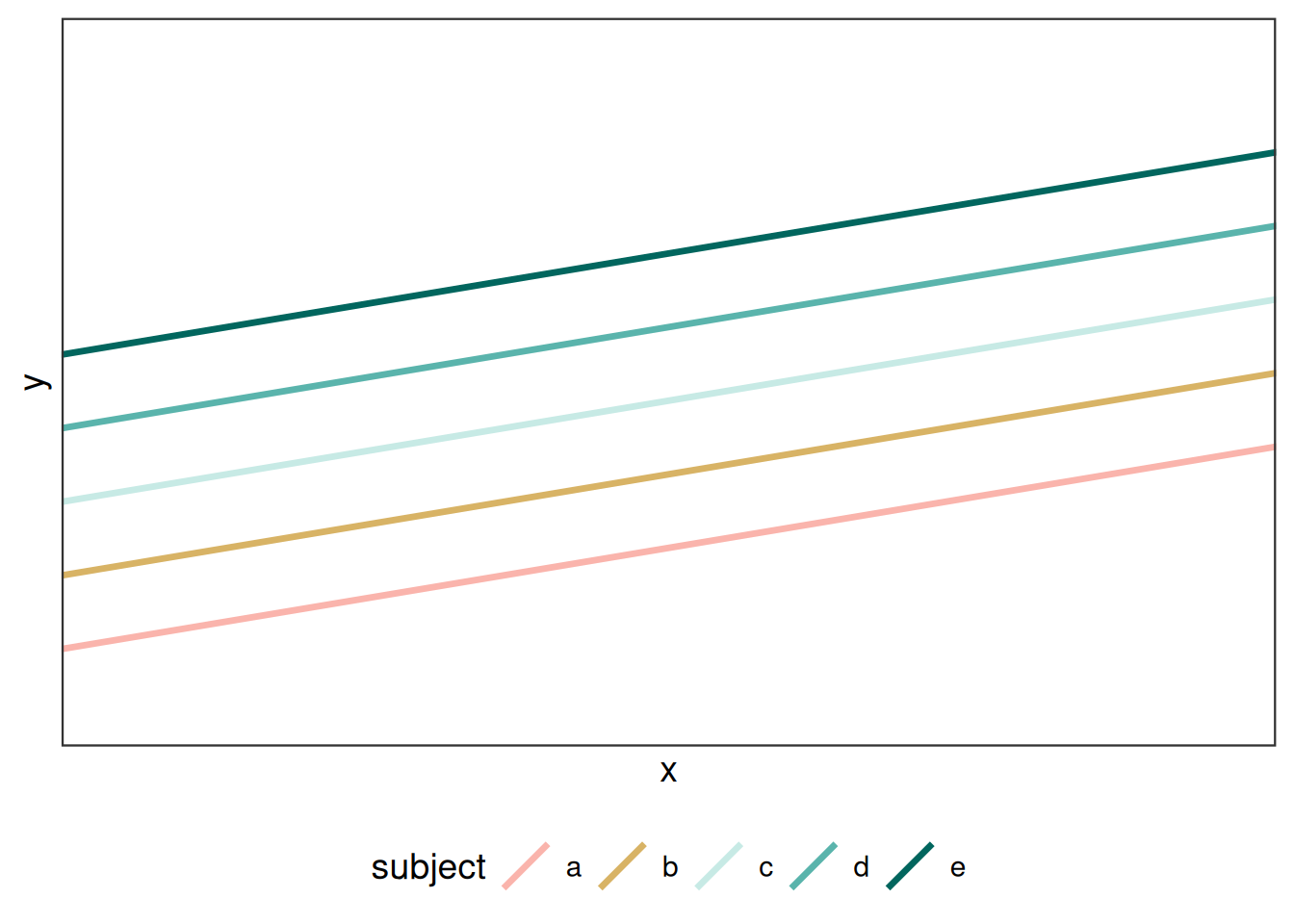
\[ Y_{ij} = \beta_0 + \beta_1 x_i + r_j + \epsilon_{ij} \] In an agronomic field trial, \(r_{j}\) could be a random effect for block (i.e. the spatial positioning of a group of treatments). Random effects are the extent of deviation due to each random unit, in this case blocks, from the model intercept, \(\beta_0\) can be thought of as each block’s deviation from the fixed intercept parameter (that is, \(\beta_0\)). Like the residuals term, \(r_i\) is independently and identically distributed (this is sometimes abbreviate “iid”):
\[r_i \sim N(0, \sigma_b)\] While random effects do not have to be normally distributed, that is the most common and most easily estimated. These are considered “random intercepts” where they all share a common slope from the fixed effects, but differ in their intercepts.
3.2.1 Random slopes models
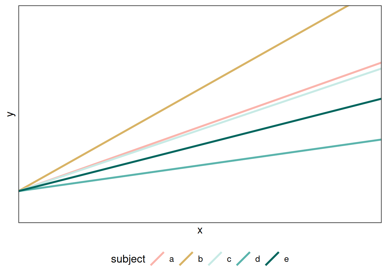
Other alternatives to the random intercept model include modelling random slopes where the slope between X and Y changes according to the random effect:
\[ Y_{ij} = \beta_0 + (\beta_1 + r_j)X_{ij} + \epsilon_{ij}\]
In this model, the \(\beta\) is the overage effect of X on Y, and \(r_i\) is a random effect for block \(j\), and all observations share a common intercept, \(\beta_0\) .
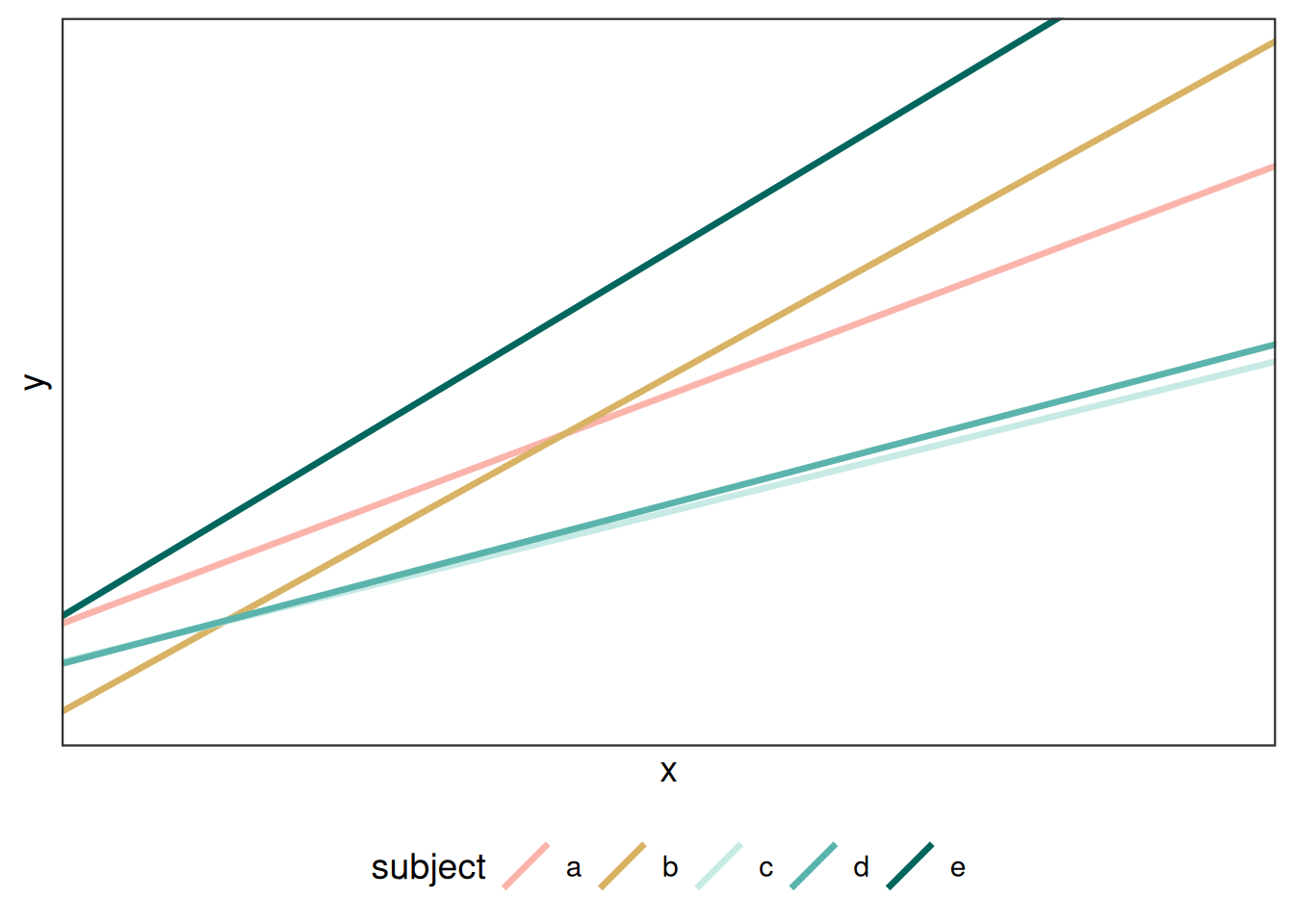
The other alternative is including both a random slope and a random intercept in the model statement:
\[ Y_{ij} = (\beta_0 + r1_j) + (\beta_1 + r1_j))X_{ij} + \epsilon_{ij}\]
In this model, \(r1_j\) and \(r1_j\) are random effects for subject \(i\) applied to the intercept and slope, respectively. These differences in slope and intercept will (likely) impact the final prediction.
This site has some nice illustrations explaining random effects.
3.3 R Formula Syntax for Random and Fixed Effects
3.3.1 lme4
The formula notation used by ‘lme4’ for the linear mixed models is as follows:
lmer(formula = Y ~ X + (1|R))In this formula, \(Y\) is the response variable (or dependent variable); \(X\) represents the independent variable(s) such as treatment (fixed effect), and \(R\) denotes the random grouping effect (e.g. block, subject).
Random effects are put in parentheses and a 1| is used to denote random intercepts (rather than random slopes). The table below ((bates?)) provides several examples of different structures for fitting random effects. The names of random grouping factors are denoted r, r1, and r2, and covariates as x.
| Formula | Alternative | Meaning |
|---|---|---|
(1|r) |
1 + (1|r) |
Random intercept with a fixed mean |
(1|r1/r2) |
(1| 1) + (1|r1:r2) |
Intercept varying among r1 and r2 within r1 |
(1|r1) + (1|r2) |
1 + (1|r1) + (1|r2) |
Intercept varying among r1 and r2 |
x + (x|r) |
1 + x + (1 + x|r) |
Correlated random intercept and slope |
x + (x||r) |
1 + x + (1|r) + (0 + x|r) |
Uncorrelated random intercept and slope |
The first example, (1|r) suffices for most mixed models and is the only structure used in this guide.
3.3.2 nlme
The package ‘nlme’ used similar notation, but the fixed and random effects are separate arguments:
lme(fixed = Y ~ X,
    random = ~ 1|R)
In this example, \(Y\), \(X\), and \(R\) are the dependent variable, fixed effect and random effect as described previously.