library(lme4); library(lmerTest); library(emmeans)
library(dplyr); library(broom.mixed); library(performance)6 RCBD Design with Several Crossed Factors
6.1 Background
Factorial designs are used when there are multiple treatments each with the multiple levels. In a full factorial, these treatments occur in all possible combinations, enabling researchers to estimate the main effect of each treatment level their interactions together on the dependent variable. Incomplete factorials are another experimental design option where some but not combinations occur in the study. This chapter focuses on the former, a full factorial study. The statistical model for a complete factorial design is:
\[y_{ijk} = \mu + \tau_i+ \beta_j + (\tau\beta)_{ij} + \delta_k + \epsilon_{ijk}\]
Where:
\(\mu\) = experiment mean
\(\tau\) = effect of factor A
\(\beta\) = effect of factor B
\(\tau\beta\) = interaction effect of factor A and B.
\(\delta\) = block effect (random)
Assumptions of this model includes: independent and identically distributed error terms with a constant variance \(\sigma^2\).
6.2 Example Analysis
First step is to load the libraries required for the analysis:
library(nlme); library(broom.mixed); library(emmeans)
library(dplyr); library(performance)
The data used in this example analysis is from the UI Department of Animal, Veterinary and Food Sciences. This trial was conducted to study the impact of two beef fabrication methods (‘trt’) in two carcass depths (‘location’) on beef top round quality. It includes 11 replications (‘animal’), where each animal was subject to all 4 possible treatment combinations. The response variable is a measure of yellowness (b_star) in the meat sample.
The objective of this example is to evaluate the individual and interactive effect of location and treatment factors on the yellowness of the meat sample.
beef <- read.csv(here::here("data/beef_factorial.csv"))| animal | random variable |
| location | location factor, 2 levels |
| trt | treatment, 2 levels |
| b_star | dependent variable |
6.2.1 Data Integrity Checks
- Check structure of the data
First step is to verify the class of variables, where animal, location, and treatment are supposed to be a factor/character and b1 should be numeric.
str(beef)'data.frame': 44 obs. of 4 variables:
$ animal : int 1 1 1 1 2 2 2 2 3 3 ...
$ location: chr "superficial" "deep" "superficial" "deep" ...
$ trt : chr "alt" "alt" "traditional" "traditional" ...
$ b_star : num 21.5 20.1 17.9 20 16.8 15.2 18.2 18.5 20.3 24.5 ...In this data, treatment factors, ‘n’, ‘p’, & ‘k’ are integers, we need to convert these variables to factor.
beef <- beef |>
mutate(animal = as.character(animal))- Inspect the independent variables
We are inspecting levels of independent variables to make sure the expected levels are present in the data.
table(beef$animal)
 1 10 11  2  3  4  5  6  7  8  9
4 4 4 4 4 4 4 4 4 4 4 table(beef$location, beef$trt)
              alt traditional
  deep         11          11
  superficial  11          11
The design looks well balanced.
- Check the extent of missing data
colSums(is.na(beef)) animal location trt b_star
0 0 0 0 There are no missing values in this data set.
- Inspect the dependent variable
This is the last step is to inspect the dependent variable to ensure it looks as expected.
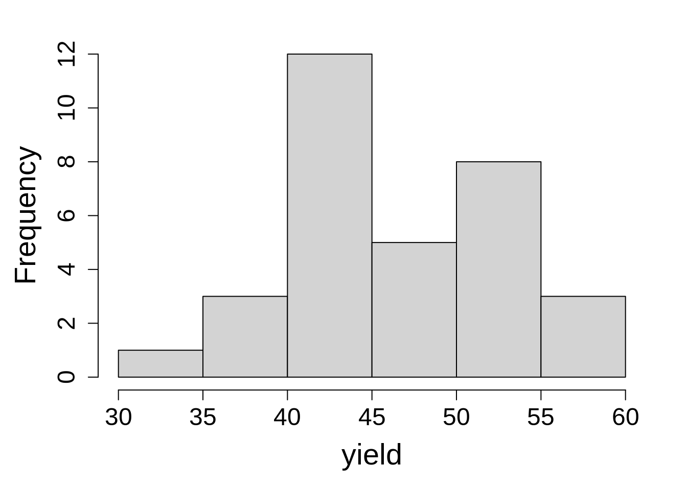
hist(beef$b_star, main = NA, xlab = "b1")No extreme values are observed in the dependent variable, and the distribution looks as expected.
6.2.2 Model Fitting
Model fitting with R is exactly the same as shown in previous chapters: we need to include all fixed effects, as well as the interaction, which is represented by using the colon, ‘:’.
The model syntax is:
b_star ~ trt + location + trt:location
which can be abbreviated as:
b_star ~ location*trt
In this analysis, location and trt are fixed factors and animal is a random effect.
mod_lmer <- lmer(b_star ~ location*trt + (1|animal),
                   data = beef,
                   na.action = na.exclude)

tidy(mod_lmer)
# A tibble: 6 × 8
effect group term estimate std.error statistic df p.value
<chr> <chr> <chr> <dbl> <dbl> <dbl> <dbl> <dbl>
1 fixed <NA> (Intercept) 19.5 0.868 22.5 24.1 1.20e-17
2 fixed <NA> locationsuperf… -2.87 0.893 -3.22 30.0 3.11e- 3
3 fixed <NA> trttraditional -1.18 0.893 -1.32 30.0 1.96e- 1
4 fixed <NA> locationsuperf… 1.81 1.26 1.43 30.0 1.62e- 1
5 ran_pars animal sd__(Intercept) 1.97 NA NA NA NA
6 ran_pars Residual sd__Observation 2.09 NA NA NA NA mod_lme <- lme(b_star ~ location*trt,
random = ~ 1|animal,
data = beef,
na.action = na.exclude)
tidy(mod_lme)# A tibble: 6 × 8
effect group term estimate std.error df statistic p.value
<chr> <chr> <chr> <dbl> <dbl> <dbl> <dbl> <dbl>
1 fixed <NA> (Intercept) 19.5 0.868 30 22.5 2.58e-20
2 fixed <NA> locationsuperf… -2.87 0.893 30 -3.22 3.11e- 3
3 fixed <NA> trttraditional -1.18 0.893 30 -1.32 1.96e- 1
4 fixed <NA> locationsuperf… 1.81 1.26 30 1.43 1.62e- 1
5 ran_pars animal sd_(Intercept) 1.97 NA NA NA NA
6 ran_pars Residual sd_Observation 2.09 NA NA NA NA
Note
The tidy() function from the ‘broom.mixed’ package provides a short summary output of the model.
6.2.3 Check Model Assumptions
check_model(mod_lmer, check = c('qq', 'linearity', 'reqq'), detrend = FALSE, alpha=0)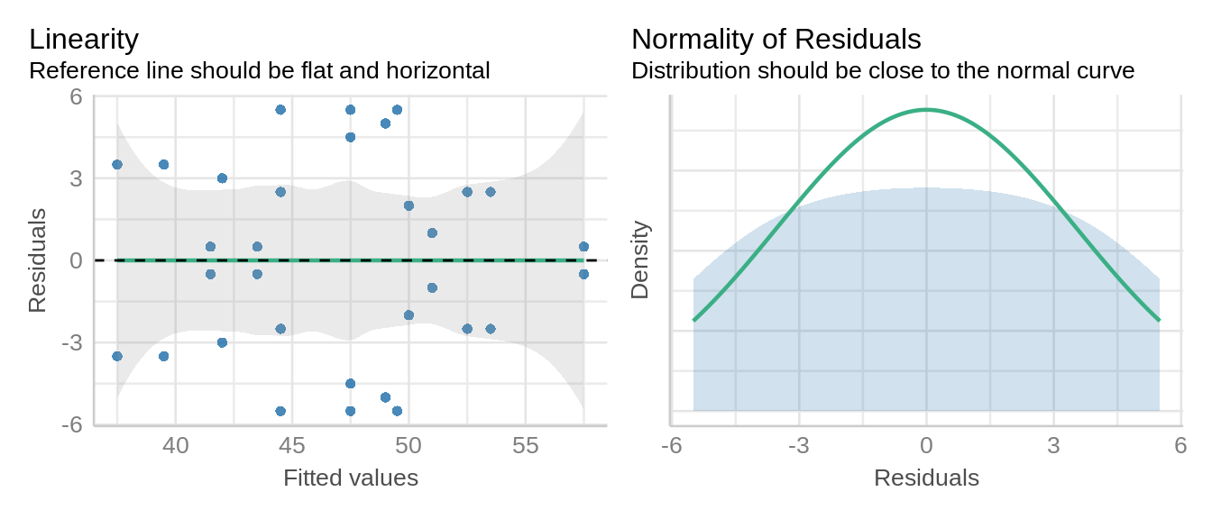
check_model(mod_lme, check = c('qq', 'linearity'), detrend = FALSE, alpha=0)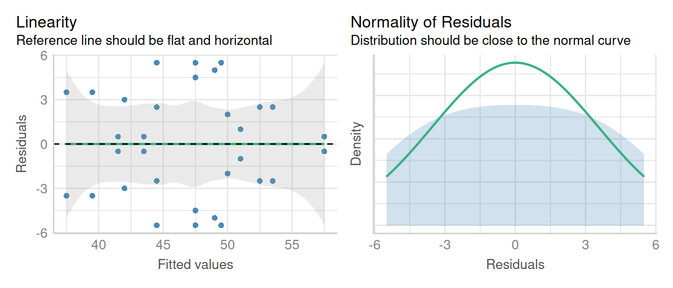
The linearity and homogeneity of variance plots show no trend. There are modest departures in the normality of residuals as indicated by the heavy tails.
6.2.4 Inference
We can obtain an ANOVA table for the linear mixed model using the function anova(), which works for both lmer() and lme() models.
anova(mod_lmer, type = "3", ddf = "Kenward-Roger")Type III Analysis of Variance Table with Kenward-Roger's method
Sum Sq Mean Sq NumDF DenDF F value Pr(>F)
location 42.611 42.611 1 30 9.7104 0.004016 **
trt 0.846 0.846 1 30 0.1927 0.663810
location:trt 9.000 9.000 1 30 2.0510 0.162442
---
Signif. codes: 0 '***' 0.001 '**' 0.01 '*' 0.05 '.' 0.1 ' ' 1anova(mod_lme, type = "marginal") numDF denDF F-value p-value
(Intercept) 1 30 504.2656 <.0001
location 1 30 10.3435 0.0031
trt 1 30 1.7506 0.1958
location:trt 1 30 2.0510 0.1624Here we do not observe any difference in group variance of interaction effects. Among all treatment factors, only location had a significant effect on the yellowness in the meat samples.
Let’s find estimates for some of the main effects and interaction effects of fixed factors on yellowness in the meat samples.
emmeans(mod_lmer, specs = ~ location)NOTE: Results may be misleading due to involvement in interactions location emmean SE df lower.CL upper.CL
deep 18.9 0.744 14.7 17.3 20.5
superficial 16.9 0.744 14.7 15.3 18.5
Results are averaged over the levels of: trt
Degrees-of-freedom method: kenward-roger
Confidence level used: 0.95 emmeans(mod_lmer, specs = ~ location)NOTE: Results may be misleading due to involvement in interactions location emmean SE df lower.CL upper.CL
deep 18.9 0.744 14.7 17.3 20.5
superficial 16.9 0.744 14.7 15.3 18.5
Results are averaged over the levels of: trt
Degrees-of-freedom method: kenward-roger
Confidence level used: 0.95 emmeans(mod_lmer, specs = ~ trt | location)location = deep:
trt emmean SE df lower.CL upper.CL
alt 19.5 0.868 24.1 17.7 21.3
traditional 18.3 0.868 24.1 16.5 20.1
location = superficial:
trt emmean SE df lower.CL upper.CL
alt 16.6 0.868 24.1 14.8 18.4
traditional 17.2 0.868 24.1 15.4 19.0
Degrees-of-freedom method: kenward-roger
Confidence level used: 0.95 emmeans(mod_lme, specs = ~ location)NOTE: Results may be misleading due to involvement in interactions location emmean SE df lower.CL upper.CL
deep 18.9 0.744 10 17.2 20.5
superficial 16.9 0.744 10 15.3 18.6
Results are averaged over the levels of: trt
Degrees-of-freedom method: containment
Confidence level used: 0.95 emmeans(mod_lme, specs = ~ trt)NOTE: Results may be misleading due to involvement in interactions trt emmean SE df lower.CL upper.CL
alt 18.0 0.744 10 16.4 19.7
traditional 17.8 0.744 10 16.1 19.4
Results are averaged over the levels of: location
Degrees-of-freedom method: containment
Confidence level used: 0.95 emmeans(mod_lme, specs = ~ trt | location)location = deep:
trt emmean SE df lower.CL upper.CL
alt 19.5 0.868 10 17.5 21.4
traditional 18.3 0.868 10 16.4 20.2
location = superficial:
trt emmean SE df lower.CL upper.CL
alt 16.6 0.868 10 14.7 18.5
traditional 17.2 0.868 10 15.3 19.2
Degrees-of-freedom method: containment
Confidence level used: 0.95 The code above is calculating the estimated marginal means for main effects of ‘trt’ within each ‘location’ under the model that includes main effects and interactions. Please note the warning message that means are averaged over the levels. It is an important detail to take into account when conducting inference and making conclusions when calculating means for a reduced model (that ignores interactions). As mentioned in many statistics courses, calculating main effects when there is an interaction present can result in misleading conclusions. When working with factorial designs, make sure to interpret ANOVA and estimated marginal means for main and interaction effects with care.