library(lme4); library(lmerTest); library(emmeans); library(performance)
library(dplyr); library(broom.mixed)11 Latin Square Design
11.1 Background
Latin square design is a spatial adjustment technique that assumes a row-by-column layout for the experimental units. Two blocking factors are are assigned, one to the rows and one for the columns of a square. This allows blocking across rows and columns to reduce the variability in those spatial units in the trial. The requirement of Latin square design is that each treatment appears only once in each row and column, and the number of replications is equal to number of treatments.
The statistical model for the Latin square design:
\(Y_{ijk} = \mu + \alpha_i + \beta_j + \gamma_k + \epsilon_{ijk}\)
where, \(\mu\) is the experiment mean, \(\alpha_i\) represents treatment effect, \(\beta\) and \(\gamma\) are the row- and column-specific effects.
Like the other designs, the residuals, \(\epsilon_{ijk}\), are assumed to independently and identically distributed, following a normal distriution. The model also assumes no interactions between the blocking factors (rows and columns) with the treatments.
11.2 Example Analysis
Let’s start the analysis first by loading the required libraries:
library(nlme); library(broom.mixed); library(emmeans); library(performance)
library(dplyr)
The data set used in this example is from the agridat package (data set “goulden.latin”). In this experiment, 5 treatments were tested to control stem rust in wheat (A = applied before rain; B = applied after rain; C = applied once each week; D = drifting once each week. E = not applied).
dat <- read.csv(here::here("data", "goulden_latin.csv"))| trt | treatment factor, 5 levels |
| row | row position for each plot |
| col | column position for each plot |
| yield | wheat yield |
11.2.1 Data Integrity Checks
- Check structure of the data
First, let’s verify the class of variables in the data set using the str() function in base R
str(dat)'data.frame': 25 obs. of 4 variables:
$ trt : chr "B" "C" "D" "E" ...
$ yield: num 4.9 9.3 7.6 5.3 9.3 6.4 4 15.4 7.6 6.3 ...
$ row : int 5 4 3 2 1 5 4 3 2 1 ...
$ col : int 1 1 1 1 1 2 2 2 2 2 ...Here yield and trt are classified as numeric and factor variables, respectively, as appropriate for their variable types. We also need to change ‘row’ and ‘col’ from integer to factor or character.
dat1 <- dat |>
        mutate(row = as.factor(row),
col = as.factor(col))- Inspect the independent variables
Next, to verify if the data meets the assumption of the Latin square design, let’s plot the field layout for this experiment.
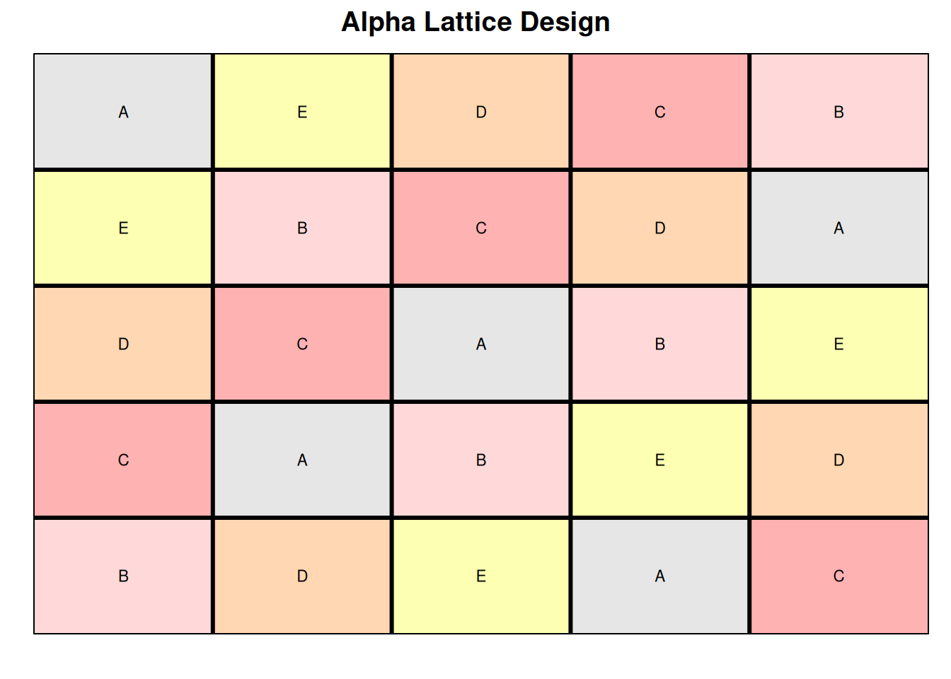
This looks as expected. Here we can see that there are an equal number of treatments, rows, and columns (5). Treatments were randomized so that one treatment does not appear more than once in each row and column.
- Check the extent of missing data
The next step is to check if there are any missing values in response variable.
colSums(is.na(dat)) trt yield row col
0 0 0 0 No missing values are detected in this data set.
- Inspect the dependent variable
Before fitting the model, let’s create a histogram of response variable to see if there are extreme values.
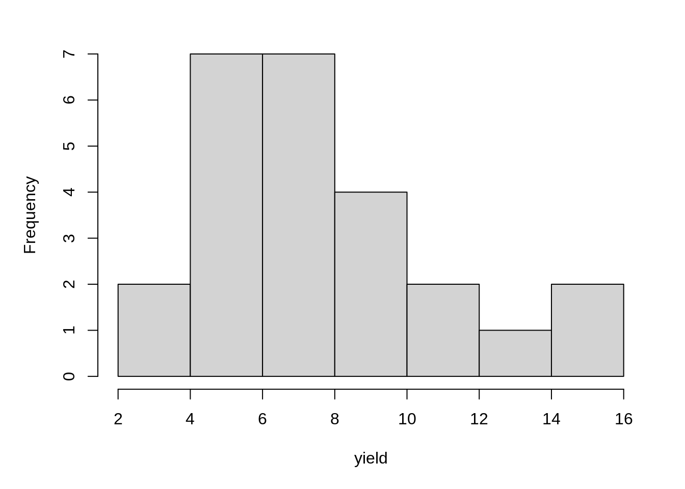
hist(dat1$yield, main = NA, xlab = "yield")11.2.2 Model Fitting
Here we will fit a model to evaluate the impact of fungicide treatments on wheat yield with trt as a fixed effect and row and col as a random effects.
m_latin_lmer <- lmer(yield ~ trt + (1|col) + (1|row),
           data = dat1,
           na.action = na.exclude)
summary(m_latin_lmer)
Linear mixed model fit by REML. t-tests use Satterthwaite's method [
lmerModLmerTest]
Formula: yield ~ trt + (1 | col) + (1 | row)
Data: dat1
REML criterion at convergence: 89.8
Scaled residuals:
Min 1Q Median 3Q Max
-1.3994 -0.5383 -0.1928 0.5220 1.8429
Random effects:
Groups Name Variance Std.Dev.
col (Intercept) 0.2336 0.4833
row (Intercept) 1.8660 1.3660
Residual 2.3370 1.5287
Number of obs: 25, groups: col, 5; row, 5
Fixed effects:
Estimate Std. Error df t value Pr(>|t|)
(Intercept) 6.8400 0.9420 11.9446 7.261 1.03e-05 ***
trtB -0.3800 0.9669 12.0000 -0.393 0.7012
trtC 6.2800 0.9669 12.0000 6.495 2.96e-05 ***
trtD 1.1200 0.9669 12.0000 1.158 0.2692
trtE -1.9200 0.9669 12.0000 -1.986 0.0704 .
---
Signif. codes: 0 '***' 0.001 '**' 0.01 '*' 0.05 '.' 0.1 ' ' 1
Correlation of Fixed Effects:
(Intr) trtB trtC trtD
trtB -0.513
trtC -0.513 0.500
trtD -0.513 0.500 0.500
trtE -0.513 0.500 0.500 0.500# this is not going well:
# dat$one <- factor(1)
# m_latin_lme <-lme(yield ~ trt,
# random = list(one = pdBlocked(list(
# pdIdent(~ 0 + row),
# pdIdent(~ 0 + col)))),
# data = dat)
# summary(m_latin_lme)
m_latin_lme1 <-lme(yield ~ trt + row,
random = ~ 1|col,
data = dat)
summary(m_latin_lme1)Linear mixed-effects model fit by REML
Data: dat
AIC BIC logLik
102.8141 110.3696 -43.40704
Random effects:
Formula: ~1 | col
(Intercept) Residual
StdDev: 0.3507367 1.699976
Fixed effects: yield ~ trt + row
Value Std.Error DF t-value p-value
(Intercept) 9.216 1.059610 15 8.697542 0.0000
trtB -0.380 1.075160 15 -0.353436 0.7287
trtC 6.280 1.075160 15 5.840994 0.0000
trtD 1.120 1.075160 15 1.041706 0.3140
trtE -1.920 1.075160 15 -1.785782 0.0944
row -0.792 0.240413 15 -3.294331 0.0049
Correlation:
(Intr) trtB trtC trtD trtE
trtB -0.507
trtC -0.507 0.500
trtD -0.507 0.500 0.500
trtE -0.507 0.500 0.500 0.500
row -0.681 0.000 0.000 0.000 0.000
Standardized Within-Group Residuals:
Min Q1 Med Q3 Max
-1.7213284 -0.2351006 -0.0850090 0.2778477 2.3767597
Number of Observations: 25
Number of Groups: 5 m_latin_lme2 <-lme(yield ~ trt + col,
random = ~ 1|row,
data = dat)
summary(m_latin_lme2)Linear mixed-effects model fit by REML
Data: dat
AIC BIC logLik
107.1628 114.7183 -45.5814
Random effects:
Formula: ~1 | row
(Intercept) Residual
StdDev: 1.331518 1.67402
Fixed effects: yield ~ trt + col
Value Std.Error DF t-value p-value
(Intercept) 6.768 1.1914188 15 5.680622 0.0000
trtB -0.380 1.0587433 15 -0.358916 0.7247
trtC 6.280 1.0587433 15 5.931560 0.0000
trtD 1.120 1.0587433 15 1.057858 0.3069
trtE -1.920 1.0587433 15 -1.813471 0.0898
col 0.024 0.2367422 15 0.101376 0.9206
Correlation:
(Intr) trtB trtC trtD trtE
trtB -0.444
trtC -0.444 0.500
trtD -0.444 0.500 0.500
trtE -0.444 0.500 0.500 0.500
col -0.596 0.000 0.000 0.000 0.000
Standardized Within-Group Residuals:
Min Q1 Med Q3 Max
-1.4090386 -0.5945754 -0.2589987 0.5933308 1.8832920
Number of Observations: 25
Number of Groups: 5 11.2.2.0.1 Latin Square Design in nlme
There is no good way (that we know of) to analyze a latin square design with nlme specifiying both row and column as random effects. One easy workaround is to only include one spatial components as random and the other as fixed. The overall estimates tend to be quite similar between models, but the variance-covariance matrices differ between models, which impacts the standard error of the estimates and any downstream comparisons made. In this case, I choose the model whose spatial component had the largest variance (row, ‘m_latin_lme2’), while also meeting standard linear modeling assumptions.
11.2.3 Check Model Assumptions
Evaluate model residuals by using check_model() function from the performance package.
check_model(m_latin_lmer, check = c('qq', 'linearity', 'reqq'), detrend = FALSE, alpha = 0)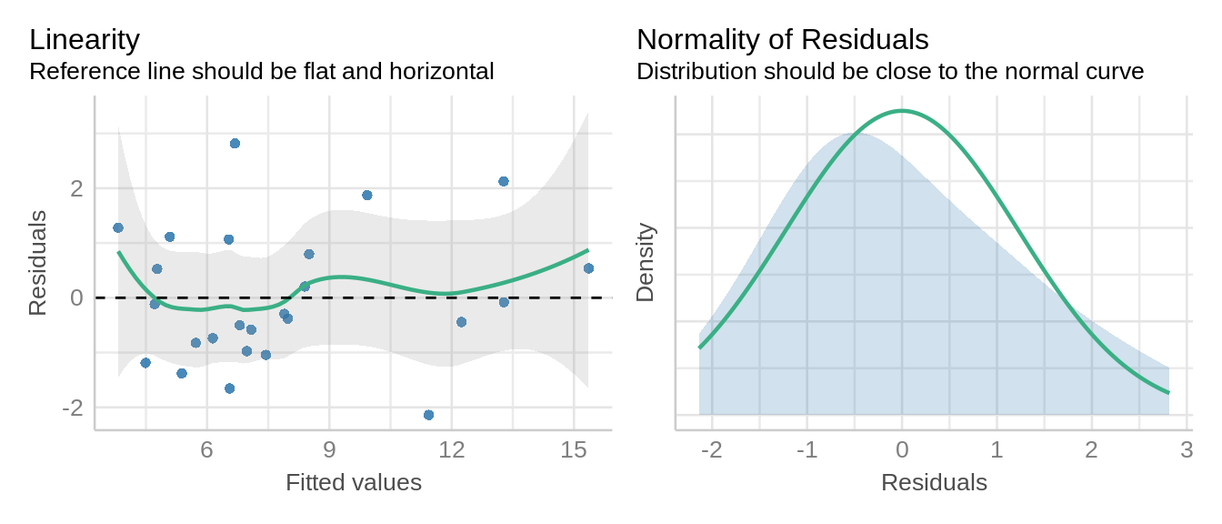
plot(m_latin_lme1, resid(., scaled=TRUE) ~ fitted(.), abline = 0,
     xlab = "fitted values", ylab = "studentized residuals")
plot(m_latin_lme2, resid(., scaled=TRUE) ~ fitted(.), abline = 0,
     xlab = "fitted values", ylab = "studentized residuals")
qqnorm(residuals(m_latin_lme1)); qqline(residuals(m_latin_lme1))
qqnorm(residuals(m_latin_lmer)); qqline(residuals(m_latin_lmer))
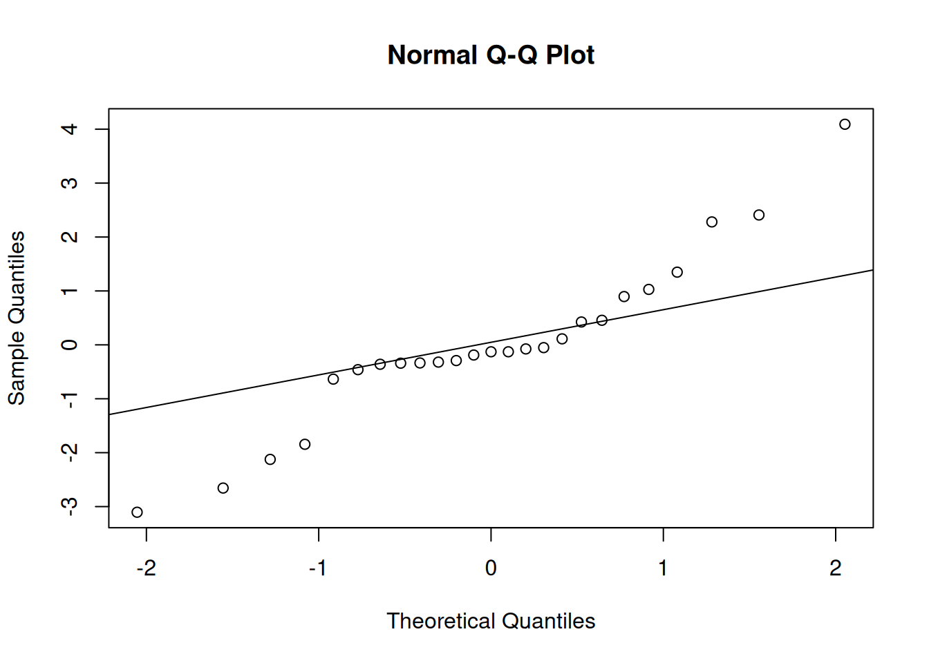
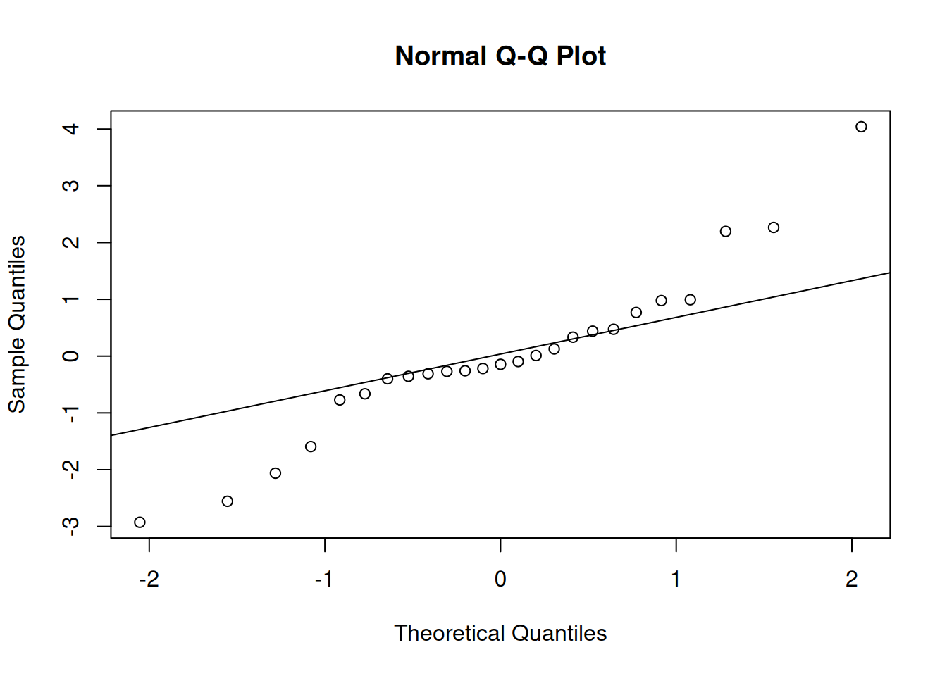
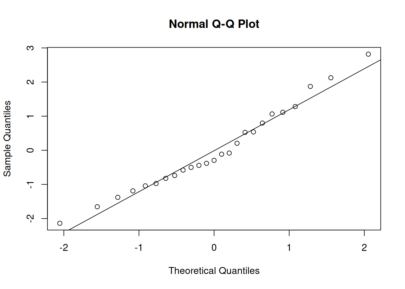
These visuals indicate that the assumptions of the linear model have been met.
11.2.4 Inference
We can now proceed with ANOVA. With only one independent variable in the model, it is immaterial what “sums of squares” type is used.
anova(m_latin_lmer)Type III Analysis of Variance Table with Satterthwaite's method
Sum Sq Mean Sq NumDF DenDF F value Pr(>F)
trt 196.61 49.152 4 12 21.032 2.366e-05 ***
---
Signif. codes: 0 '***' 0.001 '**' 0.01 '*' 0.05 '.' 0.1 ' ' 1anova(m_latin_lme2) numDF denDF F-value p-value
(Intercept) 1 15 132.38053 <.0001
trt 4 15 17.53961 <.0001
col 1 15 0.01028 0.9206Here we observed a statistically significant impact of fungicide treatment on crop yield. Let’s have a look at the estimated marginal means of wheat yield with each treatment using the emmeans() function.
emmeans(m_latin_lmer, ~ trt) trt emmean SE df lower.CL upper.CL
A 6.84 0.942 11.9 4.79 8.89
B 6.46 0.942 11.9 4.41 8.51
C 13.12 0.942 11.9 11.07 15.17
D 7.96 0.942 11.9 5.91 10.01
E 4.92 0.942 11.9 2.87 6.97
Degrees-of-freedom method: kenward-roger
Confidence level used: 0.95 emmeans(m_latin_lme2, ~ trt) trt emmean SE df lower.CL upper.CL
A 6.84 0.957 4 4.18 9.50
B 6.46 0.957 4 3.80 9.12
C 13.12 0.957 4 10.46 15.78
D 7.96 0.957 4 5.30 10.62
E 4.92 0.957 4 2.26 7.58
Degrees-of-freedom method: containment
Confidence level used: 0.95 We see that wheat yield was higher with ‘C’ fungicide treatment compared to other fungicides applied in this study, indicating that ‘C’ fungicide was more effective in controlling stem rust in wheat.