library(lme4); library(lmerTest); library(emmeans)
library(dplyr); library(broom.mixed); library(performance)10 Incomplete Block Design
10.1 Background
The block design described in Chapter 4 was complete, meaning that each block contained each treatment level at least once. In practice, it may not be possible or advisable to include all treatments in each block, either due to limitations in treatment availability (e.g. limited seed stocks) or the block size becomes too large to serve its original goals of controlling for spatial variation.
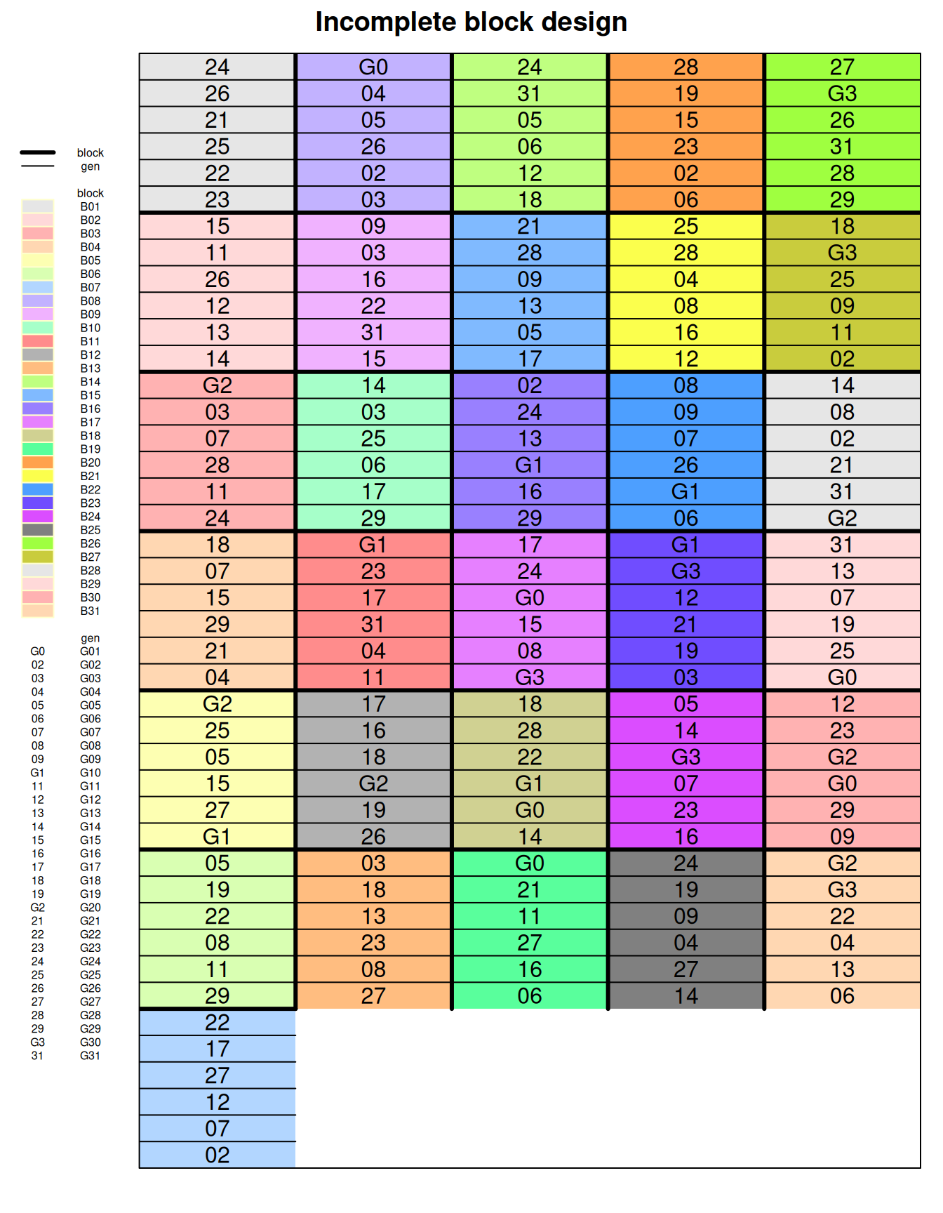
In such cases, incomplete block designs (IBD) can be used. Incomplete block designs break the experiment into many smaller incomplete blocks that are nested within standard RCBD-style blocks and assigns a subset of the treatment levels to each incomplete block. There are several different approaches (Yates 1936) for how to assign treatment levels to incomplete blocks and these designs impact the final statistical analysis (and if all treatments included in the experimental design are estimable). An excellent description of incomplete block designs is provided by Lukas Meier in ANOVA and Mixed Models (2022) and his lecture notes as well as in lecture notes by Jennifer Kling.
Incomplete block designs are grouped into two groups: (1) balanced designs; and (2) partially balanced (also commonly called alpha-lattice) designs (Oehlert 2000). Balanced IBD designs have been previously called “lattice designs” (Nair 1952), but we are not using that term to avoid confusion with alpha-lattice designs. In a balanced design, treatment pairs occur together in equal numbers for all possible pairwise treatment combinations. This enables a user to conduct all pairwise comparisons, but it not always feasible to implement, particularly when there is a large number of treatment, such as in a crop variety trial. The balanced incomplete block designs are guided by strict principles and guidelines including: the number of treatments must be a perfect square (e.g. 25, 36, and so on), and number of replicates must be equal to number of blocks + 1.
In a partially balanced design, treatment pairs occur unequally across the experiments and some pairs do not occur at all. These designs are sometimes labelled “disconnected” when all treatment pairs do not occur together because those pairwise combinations can be contrasted in a statistical analysis. In alpha-lattice design, the sub-blocks are grouped into complete replicates. The replication is considered the “superblock” consisting of multiple sub-blocks and each treatment occurs at least once. These designs are also termed as “resolvable incomplete block designs” (Patterson and Williams 1976). This design has been more commonly used instead of balanced IBD because of it’s practicability and versatility when there is a large number of treatments. In this design, we have t treatment groups, each occurring r times, with bk experimental units groups into b blocks of size k<v in such a manner that units within a block are same and units in different blocks are substantially different.
10.1.1 Statistical Model
The statistical model for a balanced incomplete block design is:
\[y_{ij} = \mu + \alpha_i + \beta_j + \epsilon_{ij}\]
Where:
\(\mu\) = overall experimental mean
\(\alpha\) = treatment effects (fixed)
\(\beta\) = block effects (random)
\(\epsilon\) = error terms
\[ \epsilon \sim N(0, \sigma)\]
\[ \beta \sim N(0, \sigma_b)\]
There are few key points that we need to keep in mind when incomplete block experiments:
- Block can be treated as fixed (“intra-block analysis”) or random (“inter-block analysis”). When it is treated as random, the block effect also contains treatment effects.
- A drawback of this design is that the estimates have less precision compared to RCBD.
- The very nature of incomplete block design results in ‘missing’ data from the standpoint of statistical software, thus ensuring that type I and type III sums of squares are different even there is no data missing for any experimental unit in the original design.
- Contrasting treatments within blocks can remove block effects, so it helps to ensure a design contains the pairwise treatment combinations of interest to the researcher.
10.2 Examples Analyses
10.2.1 Balanced Incomplete Block Design
We will demonstrate how to analyze an example balanced incomplete block design. First, load the libraries required for analysis.
library(nlme); library(broom.mixed); library(emmeans)
library(dplyr); library(performance)
The data used for this example analysis is from the ‘agridat’ package (data set “weiss.incblock”). This example is comprised of soybean balanced incomplete block experiment.
weiss <- read.csv(here::here("data", "weiss_ICB.csv"))| block | blocking unit |
| gen | genotype (variety) factor |
| row | row position for each plot |
| col | column position for each plot |
| yield | grain yield in bu/ac |
10.2.1.1 Data integrity checks
- Check structure of the data
We will start inspecting the data set first by looking at the class of each variable:
str(weiss)'data.frame': 186 obs. of 5 variables:
$ block: chr "B01" "B02" "B03" "B04" ...
$ gen : chr "G24" "G15" "G20" "G18" ...
$ yield: num 29.8 24.2 30.5 20 35.2 25 23.6 23.6 29.3 25.5 ...
$ row : int 42 36 30 24 18 12 6 42 36 30 ...
$ col : int 1 1 1 1 1 1 1 2 2 2 ...The variables we need for the model are block, gen, and yield. The block and gen are classified as factor variables and yield is numeric. Therefore, we do not need to change class of any of the required variables.
- Inspect the independent variables
Next, let’s check the independent variables. We can look at this by running a cross tabulations among block and gen factors.
table(weiss$gen)
G01 G02 G03 G04 G05 G06 G07 G08 G09 G10 G11 G12 G13 G14 G15 G16 G17 G18 G19 G20
  6   6   6   6   6   6   6   6   6   6   6   6   6   6   6   6   6   6   6   6
G21 G22 G23 G24 G25 G26 G27 G28 G29 G30 G31
6 6 6 6 6 6 6 6 6 6 6 table(weiss$block)
B01 B02 B03 B04 B05 B06 B07 B08 B09 B10 B11 B12 B13 B14 B15 B16 B17 B18 B19 B20
  6   6   6   6   6   6   6   6   6   6   6   6   6   6   6   6   6   6   6   6
B21 B22 B23 B24 B25 B26 B27 B28 B29 B30 B31
  6   6   6   6   6   6   6   6   6   6   6
There are 31 varieties that are perfectly balanced, with exactly one observation per treatment per superblock.
- Check the extent of missing data
colSums(is.na(weiss))block gen yield row col
0 0 0 0 0 No missing data!
- Inspect the dependent variable
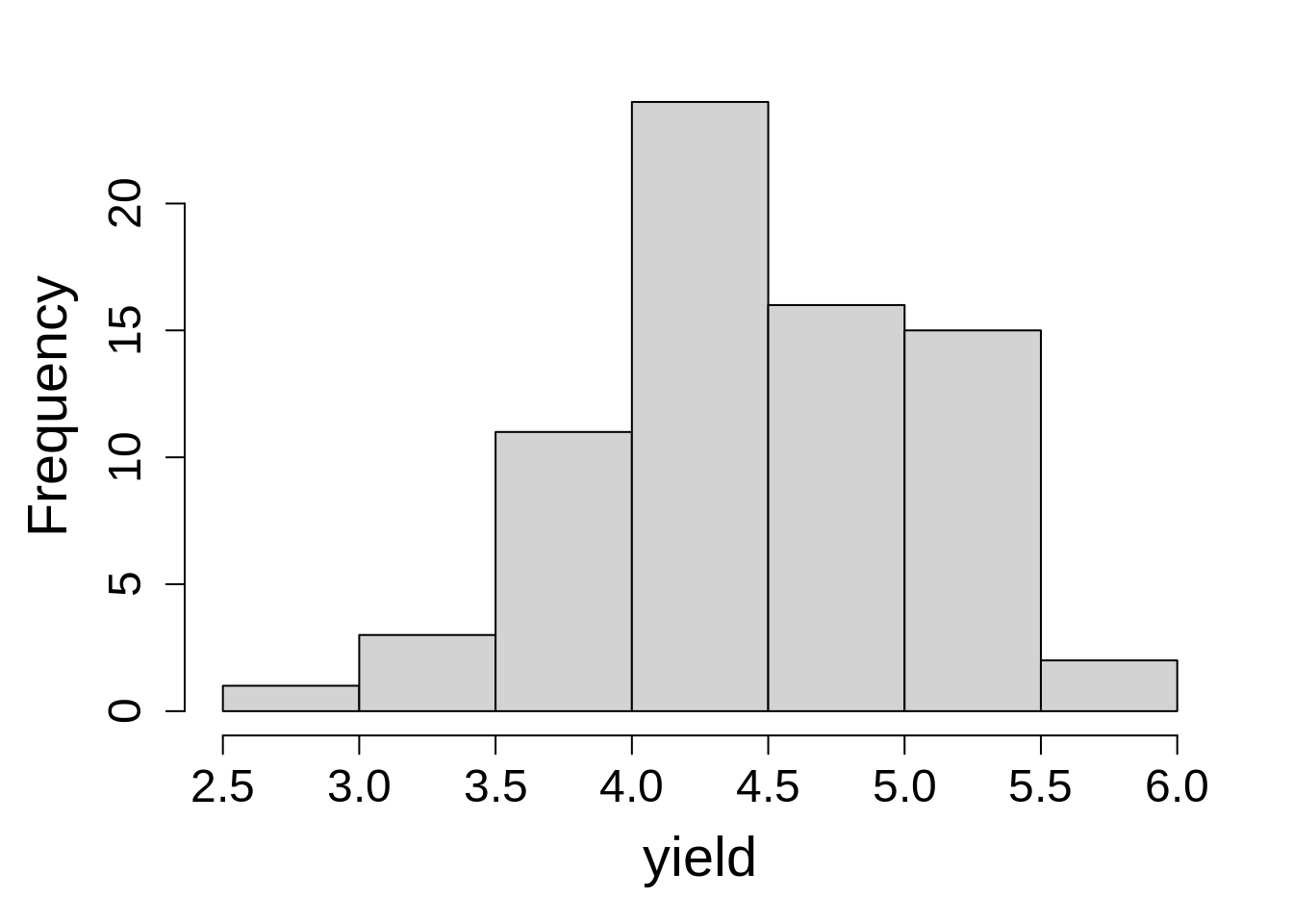
Last, let’s plot a histogram of the dependent variable. This is a quick check before analysis to see if there are any major or unexpected deviations in values.
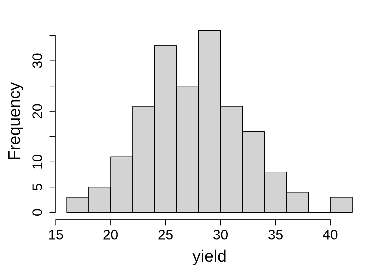
hist(weiss$yield, main = NA, xlab = "yield")Response variable values fall within expected range, with a few larger values on the right tail.
10.2.1.2 Model Building
We will be evaluating the response of yield as affected by ‘gen’ (fixed effect) and ‘block’ (random effect).
model_icbd <- lmer(yield ~ gen + (1|block),
                   data = weiss,
                   na.action = na.exclude)

model_icbd
Linear mixed model fit by REML ['lmerModLmerTest']
Formula: yield ~ gen + (1 | block)
Data: weiss
REML criterion at convergence: 757.8465
Random effects:
Groups Name Std.Dev.
block (Intercept) 2.295
Residual 1.893
Number of obs: 186, groups: block, 31
Fixed Effects:
(Intercept) genG02 genG03 genG04 genG05 genG06
24.5730 2.4031 8.0412 2.3742 1.6003 7.3903
genG07 genG08 genG09 genG10 genG11 genG12
-0.4194 3.0384 4.8380 -0.0429 2.4839 4.6862
genG13 genG14 genG15 genG16 genG17 genG18
5.3687 -0.3271 1.5156 1.3545 -4.8745 1.1513
genG19 genG20 genG21 genG22 genG23 genG24
4.4677 8.5819 6.5146 0.5986 5.2441 9.0677
genG25 genG26 genG27 genG28 genG29 genG30
2.4203 2.5629 -0.7651 1.8992 0.1897 11.6045
genG31
2.5347 model_icbd1 <- lme(yield ~ gen,
random = ~ 1|block,
data = weiss,
na.action = na.exclude)
model_icbd1Linear mixed-effects model fit by REML
Data: weiss
Log-restricted-likelihood: -378.9233
Fixed: yield ~ gen
(Intercept) genG02 genG03 genG04 genG05 genG06
24.57303855 2.40313510 8.04117318 2.37422767 1.60025683 7.39029978
genG07 genG08 genG09 genG10 genG11 genG12
-0.41940045 3.03844237 4.83798217 -0.04290217 2.48386430 4.68622645
genG13 genG14 genG15 genG16 genG17 genG18
5.36871014 -0.32706907 1.51557627 1.35453230 -4.87448450 1.15125988
genG19 genG20 genG21 genG22 genG23 genG24
4.46766255 8.58186834 6.51456431 0.59856593 5.24414300 9.06769050
genG25 genG26 genG27 genG28 genG29 genG30
2.42031071 2.56285437 -0.76507920 1.89916346 0.18974802 11.60449544
genG31
2.53465383
Random effects:
Formula: ~1 | block
(Intercept) Residual
StdDev: 2.295105 1.893486
Number of Observations: 186
Number of Groups: 31 10.2.1.3 Check Model Assumptions
Let’s verify the assumption of linear mixed models including normal distribution and constant variance of residuals.
check_model(model_icbd, check = c('qq', 'linearity', 'reqq'), detrend = FALSE, alpha = 0)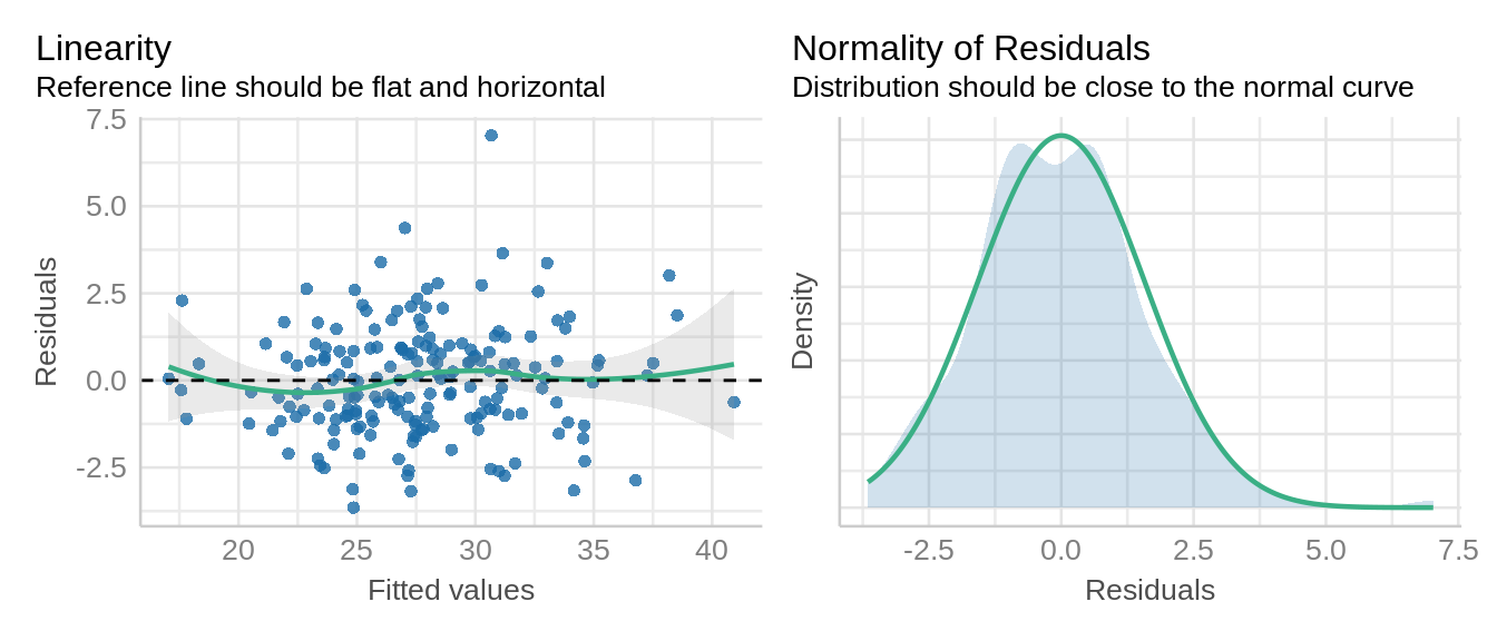
check_model(model_icbd1, check = c('qq', 'linearity'), detrend = FALSE, alpha = 0)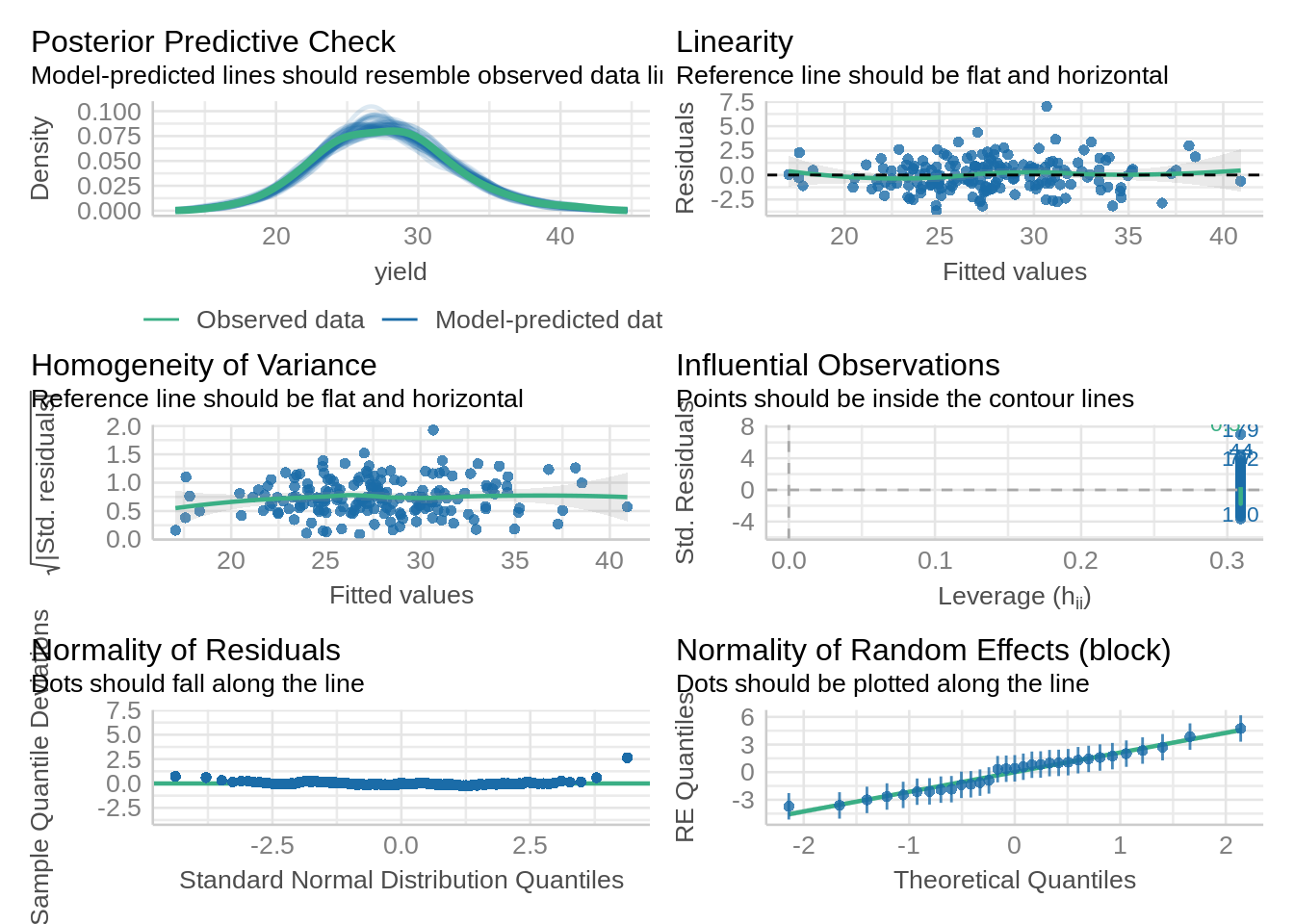
10.2.1.4 Inference
We can extract information about ANOVA using anova().
anova(model_icbd, type = "1")Type I Analysis of Variance Table with Satterthwaite's method
Sum Sq Mean Sq NumDF DenDF F value Pr(>F)
gen 1901.1 63.369 30 129.06 17.675 < 2.2e-16 ***
---
Signif. codes: 0 '***' 0.001 '**' 0.01 '*' 0.05 '.' 0.1 ' ' 1anova(model_icbd1, type = "sequential") numDF denDF F-value p-value
(Intercept) 1 125 4042.016 <.0001
gen 30 125 17.675 <.0001Let’s look at the estimated marginal means of yield for each variety (gen).
emmeans(model_icbd, ~ gen) gen emmean SE df lower.CL upper.CL
G01 24.6 0.923 153 22.7 26.4
G02 27.0 0.923 153 25.2 28.8
G03 32.6 0.923 153 30.8 34.4
G04 26.9 0.923 153 25.1 28.8
G05 26.2 0.923 153 24.4 28.0
G06 32.0 0.923 153 30.1 33.8
G07 24.2 0.923 153 22.3 26.0
G08 27.6 0.923 153 25.8 29.4
G09 29.4 0.923 153 27.6 31.2
G10 24.5 0.923 153 22.7 26.4
G11 27.1 0.923 153 25.2 28.9
G12 29.3 0.923 153 27.4 31.1
G13 29.9 0.923 153 28.1 31.8
G14 24.2 0.923 153 22.4 26.1
G15 26.1 0.923 153 24.3 27.9
G16 25.9 0.923 153 24.1 27.8
G17 19.7 0.923 153 17.9 21.5
G18 25.7 0.923 153 23.9 27.5
G19 29.0 0.923 153 27.2 30.9
G20 33.2 0.923 153 31.3 35.0
G21 31.1 0.923 153 29.3 32.9
G22 25.2 0.923 153 23.3 27.0
G23 29.8 0.923 153 28.0 31.6
G24 33.6 0.923 153 31.8 35.5
G25 27.0 0.923 153 25.2 28.8
G26 27.1 0.923 153 25.3 29.0
G27 23.8 0.923 153 22.0 25.6
G28 26.5 0.923 153 24.6 28.3
G29 24.8 0.923 153 22.9 26.6
G30 36.2 0.923 153 34.4 38.0
G31 27.1 0.923 153 25.3 28.9
Degrees-of-freedom method: kenward-roger
Confidence level used: 0.95 emmeans(model_icbd1, ~ gen) gen emmean SE df lower.CL upper.CL
G01 24.6 0.922 30 22.7 26.5
G02 27.0 0.922 30 25.1 28.9
G03 32.6 0.922 30 30.7 34.5
G04 26.9 0.922 30 25.1 28.8
G05 26.2 0.922 30 24.3 28.1
G06 32.0 0.922 30 30.1 33.8
G07 24.2 0.922 30 22.3 26.0
G08 27.6 0.922 30 25.7 29.5
G09 29.4 0.922 30 27.5 31.3
G10 24.5 0.922 30 22.6 26.4
G11 27.1 0.922 30 25.2 28.9
G12 29.3 0.922 30 27.4 31.1
G13 29.9 0.922 30 28.1 31.8
G14 24.2 0.922 30 22.4 26.1
G15 26.1 0.922 30 24.2 28.0
G16 25.9 0.922 30 24.0 27.8
G17 19.7 0.922 30 17.8 21.6
G18 25.7 0.922 30 23.8 27.6
G19 29.0 0.922 30 27.2 30.9
G20 33.2 0.922 30 31.3 35.0
G21 31.1 0.922 30 29.2 33.0
G22 25.2 0.922 30 23.3 27.1
G23 29.8 0.922 30 27.9 31.7
G24 33.6 0.922 30 31.8 35.5
G25 27.0 0.922 30 25.1 28.9
G26 27.1 0.922 30 25.3 29.0
G27 23.8 0.922 30 21.9 25.7
G28 26.5 0.922 30 24.6 28.4
G29 24.8 0.922 30 22.9 26.6
G30 36.2 0.922 30 34.3 38.1
G31 27.1 0.922 30 25.2 29.0
Degrees-of-freedom method: containment
Confidence level used: 0.95 10.2.2 Partially Balanced IBD (Alpha Lattice Design)
The statistical model for partially balanced design includes:
\[y_{ij(l)} = \mu + \alpha_i + \beta_{i(l)} + \tau_j + \epsilon_{ij(l)}\]
Where:
\(\mu\) = overall experimental mean
\(\alpha\) = replicate effect (random)
\(\beta\) = incomplete block effect (random)
\(\tau\) = treatment effect (fixed)
\(\epsilon_{ij(l)}\) = intra-block residual
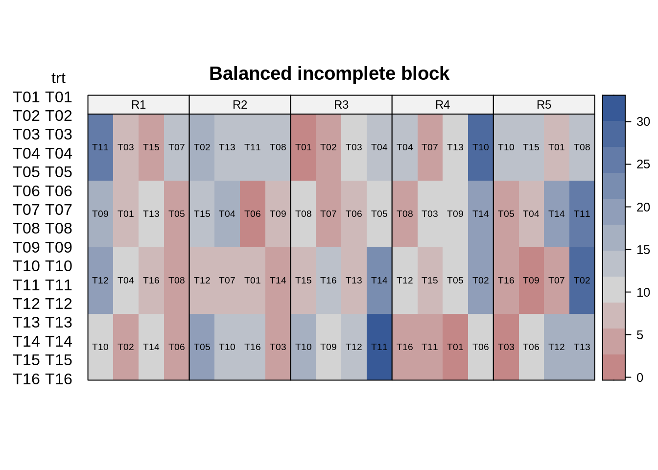
The data used in this example is published in Cyclic and Computer Generated Designs (John and Williams 1995). The trial was laid out in an alpha lattice design. This trial data had 24 genotypes (“gen”), 6 incomplete blocks, each replicated 3 times.
Let’s start analyzing this example first by loading the required libraries for linear mixed models:
library(lme4); library(lmerTest); library(emmeans)
library(dplyr); library(broom.mixed); library(performance)library(nlme); library(broom.mixed); library(emmeans)
library(dplyr); library(performance)Let’s import a data with partial balanced icomplete design. This data set, ‘john.alpha’, describes a spring oats study and was obtained from the ‘agridat’ package.
p_icb <- read.csv(here::here("data", "partial_incblock.csv"))| block | incomplete blocking unit |
| gen | genotype (variety) factor |
| row | row position for each plot |
| col | column position for each plot |
| yield | grain yield in tonnes/ha |
10.2.2.1 Data integrity checks
- Check structure of the data
Let’s look into the structure of the data first to verify the class of the variables.
str(p_icb)'data.frame': 72 obs. of 7 variables:
$ plot : int 1 2 3 4 5 6 7 8 9 10 ...
$ rep : chr "R1" "R1" "R1" "R1" ...
$ block: chr "B1" "B1" "B1" "B1" ...
$ gen : chr "G11" "G04" "G05" "G22" ...
$ yield: num 4.12 4.45 5.88 4.58 4.65 ...
$ row : int 1 2 3 4 5 6 7 8 9 10 ...
$ col : int 1 1 1 1 1 1 1 1 1 1 ...Here, ‘rep’, ‘block’, and ‘gen’ are character variables and ’yield’is formatted as numeric, all correct formats for downstream analysis.
- Inspect the independent variables
The next step is to checkl the independent variables. First, check the number of treatments per replication (each treatment should be replicated 3 times).
table(p_icb$gen)
G01 G02 G03 G04 G05 G06 G07 G08 G09 G10 G11 G12 G13 G14 G15 G16 G17 G18 G19 G20
  3   3   3   3   3   3   3   3   3   3   3   3   3   3   3   3   3   3   3   3
G21 G22 G23 G24
  3   3   3   3
This looks balanced, as expected. Also, let’s have a look at the number of times each treatment appear per block.
table(p_icb$block)
B1 B2 B3 B4 B5 B6
12 12 12 12 12 12
12 treatments randomly occur in each incomplete block, and each incomplete block has same number of treatments.
- Check the extent of missing data
colSums(is.na(p_icb)) plot rep block gen yield row col
0 0 0 0 0 0 0 There are no missing values in the data set.
- Inspect the dependent variable
Before fitting the model, it’s a good idea to look at the distribution of dependent variable, yield.
hist(p_icb$yield, main = NA, xlab = "yield")The response variables seems to follow a normal distribution curve, with few values on extreme lower and higher ends.
10.2.2.2 Model Building
We are evaluating the response of ‘yield’ to ‘Gen’ (a fixed effect) and ‘rep’ and ‘block’ as random effects.
mod_alpha <- lmer(yield ~ gen + (1|rep/block),
                   data = p_icb,
                   na.action = na.exclude)

mod_alpha
Linear mixed model fit by REML ['lmerModLmerTest']
Formula: yield ~ gen + (1 | rep/block)
Data: p_icb
REML criterion at convergence: 67.5586
Random effects:
Groups Name Std.Dev.
block:rep (Intercept) 0.2489
rep (Intercept) 0.3376
Residual 0.2919
Number of obs: 72, groups: block:rep, 18; rep, 3
Fixed Effects:
(Intercept) genG02 genG03 genG04 genG05 genG06
5.10770 -0.62917 -1.60850 -0.61761 -0.07049 -0.57104
genG07 genG08 genG09 genG10 genG11 genG12
-0.99656 -0.58007 -1.60552 -0.73450 -0.82444 -0.35242
genG13 genG14 genG15 genG16 genG17 genG18
-0.34979 -0.33204 -0.13859 -0.37757 -0.50509 -0.74601
genG19 genG20 genG21 genG22 genG23 genG24
-0.26737 -1.06772 -0.31269 -0.58015 -0.85525 -0.95383 mod_alpha1 <- lme(yield ~ gen,
random = ~ 1|rep/block,
data = p_icb,
na.action = na.exclude)
mod_alpha1Linear mixed-effects model fit by REML
Data: p_icb
Log-restricted-likelihood: -33.7793
Fixed: yield ~ gen
(Intercept) genG02 genG03 genG04 genG05 genG06
5.1076995 -0.6291674 -1.6084999 -0.6176050 -0.0704892 -0.5710374
genG07 genG08 genG09 genG10 genG11 genG12
-0.9965634 -0.5800658 -1.6055185 -0.7345000 -0.8244354 -0.3524231
genG13 genG14 genG15 genG16 genG17 genG18
-0.3497863 -0.3320375 -0.1385881 -0.3775685 -0.5050871 -0.7460071
genG19 genG20 genG21 genG22 genG23 genG24
-0.2673717 -1.0677145 -0.3126921 -0.5801548 -0.8552508 -0.9538255
Random effects:
Formula: ~1 | rep
(Intercept)
StdDev: 0.3375614
Formula: ~1 | block %in% rep
(Intercept) Residual
StdDev: 0.2488852 0.2919334
Number of Observations: 72
Number of Groups:
rep block %in% rep
3 18 10.2.2.3 Check Model Assumptions
Let’s verify the assumption of linear mixed models (normal distribution and constant variance of residuals).
check_model(mod_alpha, check = c('qq', 'linearity', 'reqq'), detrend = FALSE, alpha = 0)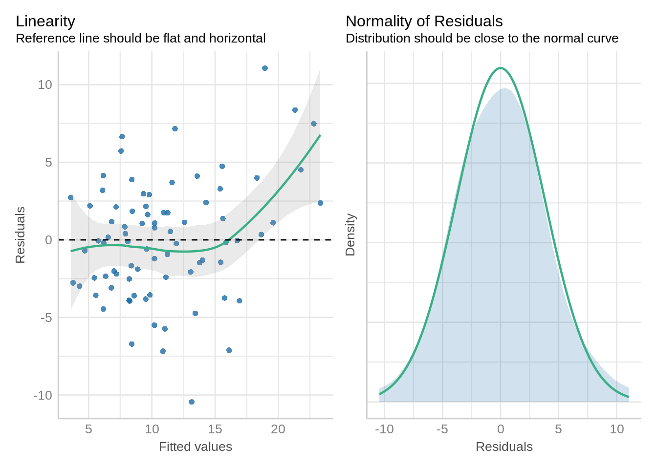
check_model(mod_alpha1, check = c('qq', 'linearity'), detrend = FALSE, alpha = 0)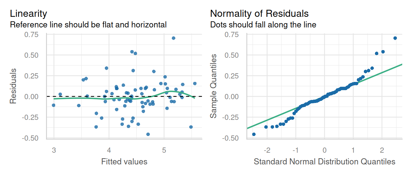
While there is some skewness present in the qq-plot, this is a minor deviation in the model assumption of normality and unlikely to impact the final results.
10.2.2.4 Inference
Let’s look at the ANOVA table using anova() from lmer and lme models, respectively.
anova(mod_alpha, type = "1")Type I Analysis of Variance Table with Satterthwaite's method
Sum Sq Mean Sq NumDF DenDF F value Pr(>F)
gen 10.679 0.46429 23 34.902 5.4478 4.229e-06 ***
---
Signif. codes: 0 '***' 0.001 '**' 0.01 '*' 0.05 '.' 0.1 ' ' 1anova(mod_alpha1, type = "sequential") numDF denDF F-value p-value
(Intercept) 1 31 470.9507 <.0001
gen 23 31 5.4478 <.0001Let’s look at the estimated marginal means of yield for each variety (gen).
emmeans(mod_alpha, ~ gen) gen emmean SE df lower.CL upper.CL
G01 5.11 0.279 6.20 4.43 5.78
G02 4.48 0.279 6.20 3.80 5.15
G03 3.50 0.279 6.20 2.82 4.18
G04 4.49 0.279 6.20 3.81 5.17
G05 5.04 0.278 6.19 4.36 5.71
G06 4.54 0.278 6.19 3.86 5.21
G07 4.11 0.279 6.20 3.43 4.79
G08 4.53 0.279 6.20 3.85 5.20
G09 3.50 0.278 6.19 2.83 4.18
G10 4.37 0.279 6.20 3.70 5.05
G11 4.28 0.279 6.20 3.61 4.96
G12 4.76 0.279 6.20 4.08 5.43
G13 4.76 0.278 6.19 4.08 5.43
G14 4.78 0.278 6.19 4.10 5.45
G15 4.97 0.278 6.19 4.29 5.65
G16 4.73 0.279 6.20 4.05 5.41
G17 4.60 0.278 6.19 3.93 5.28
G18 4.36 0.279 6.20 3.69 5.04
G19 4.84 0.278 6.19 4.16 5.52
G20 4.04 0.278 6.19 3.36 4.72
G21 4.80 0.278 6.19 4.12 5.47
G22 4.53 0.278 6.19 3.85 5.20
G23 4.25 0.278 6.19 3.58 4.93
G24 4.15 0.279 6.20 3.48 4.83
Degrees-of-freedom method: kenward-roger
Confidence level used: 0.95 emmeans(mod_alpha1, ~ gen) gen emmean SE df lower.CL upper.CL
G01 5.11 0.276 2 3.92 6.30
G02 4.48 0.276 2 3.29 5.67
G03 3.50 0.276 2 2.31 4.69
G04 4.49 0.276 2 3.30 5.68
G05 5.04 0.276 2 3.85 6.22
G06 4.54 0.276 2 3.35 5.72
G07 4.11 0.276 2 2.92 5.30
G08 4.53 0.276 2 3.34 5.72
G09 3.50 0.276 2 2.31 4.69
G10 4.37 0.276 2 3.19 5.56
G11 4.28 0.276 2 3.10 5.47
G12 4.76 0.276 2 3.57 5.94
G13 4.76 0.276 2 3.57 5.95
G14 4.78 0.276 2 3.59 5.96
G15 4.97 0.276 2 3.78 6.16
G16 4.73 0.276 2 3.54 5.92
G17 4.60 0.276 2 3.42 5.79
G18 4.36 0.276 2 3.17 5.55
G19 4.84 0.276 2 3.65 6.03
G20 4.04 0.276 2 2.85 5.23
G21 4.80 0.276 2 3.61 5.98
G22 4.53 0.276 2 3.34 5.72
G23 4.25 0.276 2 3.06 5.44
G24 4.15 0.276 2 2.97 5.34
Degrees-of-freedom method: containment
Confidence level used: 0.95 The estimates are identical across ‘nlme’ and ‘lme4’, but the standard errors differ slightly. The degrees of freedom differ greatly due to the different approaches used for esimating those, impacting the confidence intervals.