library(lme4); library(lmerTest); library(emmeans)
library(dplyr); library(performance)5 Randomized Complete Block Design
Randomized complete block design (RCBD) is very common design where experimental treatments are applied at random to experimental units within each block. The block can represent a spatial or temporal unit or even different technicians taking data. The blocks are intended to control for a nuisance source of variation, such as time, spatial variation, changes in equipment or operators, or myriad other causes. They are a random effect where the ‘blocks’ used in the study are a random sample from a distribution of other blocks.
5.1 Background
The statistical model:
\[y_{ij} = \mu + \alpha_i + \beta_j + \epsilon_{ij}\]
Where:
\(\mu\) = overall experimental mean
\(\alpha\) = treatment effects (fixed)
$ = block effects (random)
and
\(\epsilon\) = error terms
\[ \epsilon \sim N(0, \sigma)\]
\[ \beta \sim N(0, \sigma_b)\]
Both the overall error and the block effects are assumed to be normally distributed with a mean of zero and standard deviations of \(\sigma\) and \(\sigma_B\), respectively.
5.2 Example Analysis
First, load the libraries for analysis and estimation:
library(nlme); library(performance); library(emmeans)
library(dplyr)
This data set is for a single wheat variety trial conducted in Aberdeen, Idaho in 2015. The trial includes 4 blocks and 42 different treatments (wheat varieties in this case). This experiment consists of a series of plots (the experimental unit) laid out in a rectangular grid in a farm field. The goal of this analysis is the estimate the yield of each variety and the determine the relative rankings of the varieties.
var_trial <- read.csv(here::here("data", "aberdeen2015.csv"))| block | blocking unit |
| range | column position for each plot |
| row | row position for each plot |
| variety | crop variety (the treatment) being evaluated |
| yield_bu_a | yield (bushels per acre) |
5.2.1 Data integrity checks
The first thing is to make sure the data is what we expect. We will follow the steps outline in Chapter 4.
- Check the structure of the data
str(var_trial)'data.frame': 168 obs. of 5 variables:
$ block : int 4 4 4 4 4 4 4 4 4 4 ...
$ range : int 1 1 1 1 1 1 1 1 1 1 ...
$ row : int 1 2 3 4 5 6 7 8 9 10 ...
$ variety : chr "DAS004" "Kaseberg" "Bruneau" "OR2090473" ...
$ yield_bu_a: num 128 130 119 115 141 ...These look okay except for block, which is currently coded as integer (a simplified numeric type). We don’t want run a regression of block, where block 2 has twice the effect of block 1, and so on. So, converting it to a character will avoid that. Block can also be converted to a factor, but character variables are a bit easier to work with, and ultimately, equivalent to factor conversion since the linear modelling functions from ‘lme4’ and ‘nlme’ automatically convert character variables to factors.
var_trial$block <- as.character(var_trial$block)- Inspect the independent variables
Next, check the independent variables. Running a cross tabulations is usually sufficient to ascertain this.
table(var_trial$variety, var_trial$block)
                         1 2 3 4
  06-03303B              1 1 1 1
  Bobtail                1 1 1 1
  Brundage               1 1 1 1
  Bruneau                1 1 1 1
  DAS003                 1 1 1 1
  DAS004                 1 1 1 1
  Eltan                  1 1 1 1
  IDN-01-10704A          1 1 1 1
  IDN-02-29001A          1 1 1 1
  IDO1004                1 1 1 1
  IDO1005                1 1 1 1
  Jasper                 1 1 1 1
  Kaseberg               1 1 1 1
  LCS Artdeco            1 1 1 1
  LCS Biancor            1 1 1 1
  LCS Drive              1 1 1 1
  LOR-833                1 1 1 1
  LOR-913                1 1 1 1
  LOR-978                1 1 1 1
  Madsen                 1 1 1 1
  Madsen / Eltan (50/50) 1 1 1 1
  Mary                   1 1 1 1
  Norwest Duet           1 1 1 1
  Norwest Tandem         1 1 1 1
  OR2080637              1 1 1 1
  OR2080641              1 1 1 1
  OR2090473              1 1 1 1
  OR2100940              1 1 1 1
  Rosalyn                1 1 1 1
  Stephens               1 1 1 1
  SY  Ovation            1 1 1 1
  SY 107                 1 1 1 1
  SY Assure              1 1 1 1
  UI Castle CLP          1 1 1 1
  UI Magic CLP           1 1 1 1
  UI Palouse             1 1 1 1
  UI Sparrow             1 1 1 1
  UI-WSU Huffman         1 1 1 1
  WB 456                 1 1 1 1
  WB 528                 1 1 1 1
  WB1376 CLP             1 1 1 1
  WB1529                 1 1 1 1
There are 42 varieties and there appears to be no misspellings among them that might confuse R into thinking varieties are different when they are actually the same. R is sensitive to case (capitalization) and white space, which can make it easy to create near duplicate treatments, such as “eltan”, “Eltan” and “Eltan”. Thankfully, there is no evidence of that in this data set. Additionally, it is perfectly balanced, with exactly one observation per treatment per rep. Please note that this does not tell us anything about the extent of missing data for individual dependent variables.
- Check the extent of missing data
Here is a quick check to count the number of missing data in each column.
colSums(is.na(var_trial)) block range row variety yield_bu_a
0 0 0 0 0 Alas, no missing data.
- Inspect the dependent variable
Last, check the dependent variable by creating a histogram.
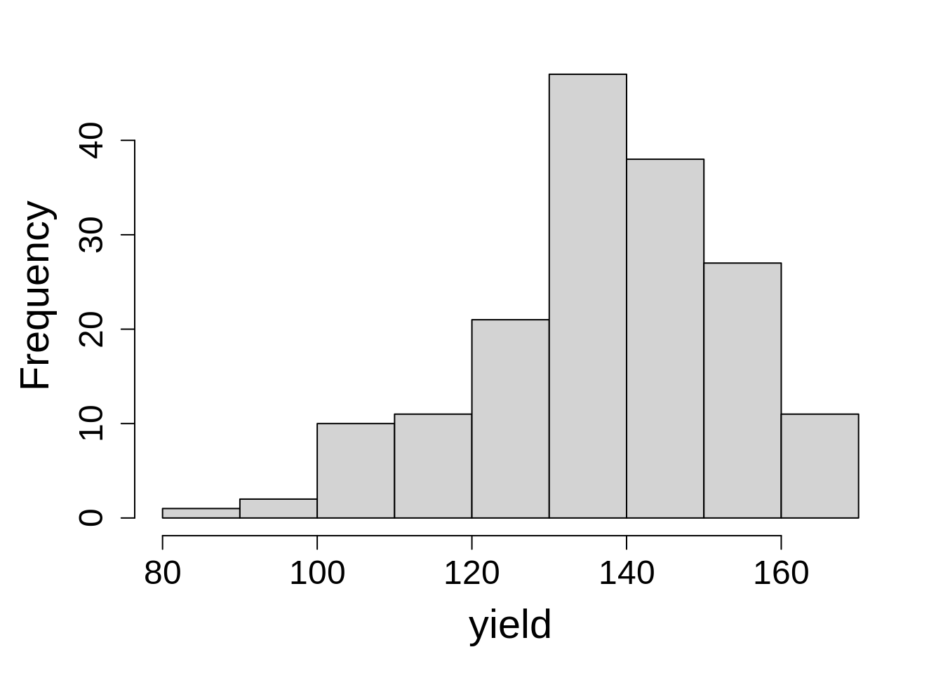
hist(var_trial$yield_bu_a, main = NA, xlab = "yield")The range of the observed data falls within the expected range of plausible values. We (the authors) know this from talking with the person who generated the data, not through our own intuition. There are no large spikes of points at a single value (indicating something odd), nor are there any extreme values (low or high) that might indicate problems that occurred during the trial or in postprocessing.
This data set is ready for analysis.
5.2.2 Model Building
Recall the model:
\[y_{ij} = \mu + \alpha_i + \beta_j + \epsilon_{ij}\]
For this model, \(\alpha_i\) is the variety effect (fixed) and \(\beta_j\) is the block effect (random).
Here is the R syntax for the RCBD statistical model:
model_rcbd_lmer <- lmer(yield_bu_a ~ variety + (1|block),
                   data = var_trial,
                   na.action = na.exclude)
model_rcbd_lme <- lme(yield_bu_a ~ variety,
random = ~ 1|block,
data = var_trial,
na.action = na.exclude)5.2.3 Check Model Assumptions
Note
R syntax for checking model assumptions is the same for lme4 and nlme package functions.
Remember those iid assumptions? Let’s make sure we actually met them.
5.2.3.1 Original Method
We will start inspecting the model assumptions by for checking the homoscedasticity (constant variance) first using a plot() function in base R.
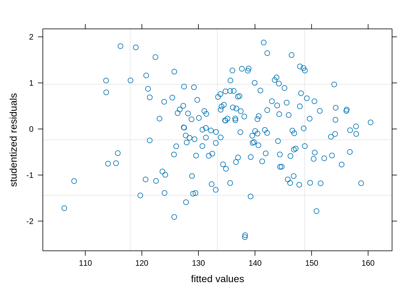
plot(model_rcbd_lmer, resid(., scaled=TRUE) ~ fitted(.),
     xlab = "fitted values", ylab = "studentized residuals")
This plot indicates a random and uniform distribution of points. Brilliant!
To make a qq plot, the residuals are extracted first and then applied to the qq plotting function.
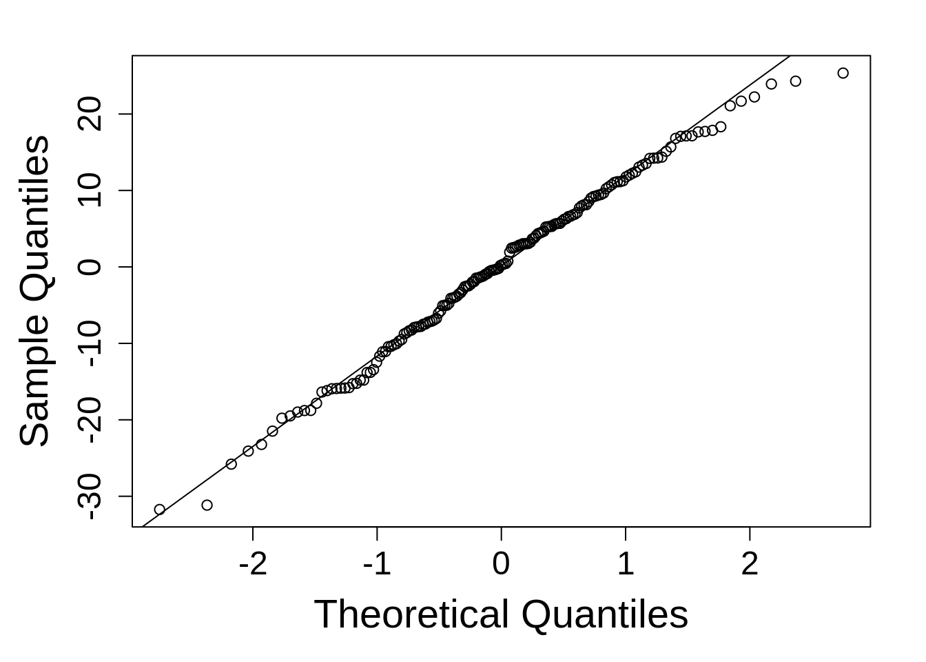
qqnorm(resid(model_rcbd_lmer), main = NULL); qqline(resid(model_rcbd_lmer))This is reasonably good. Things do tend to fall apart at the tails a little, but si nce linear models are robust to model departures from normality, this is not concerning.
5.2.3.2 New Method
Here, we will use the check_model() function from the ‘performance’ package to look at the normality and linearity of the residuals.
check_model(model_rcbd_lmer, check = c('qq', 'linearity', 'reqq'), detrend = FALSE, alpha = 0)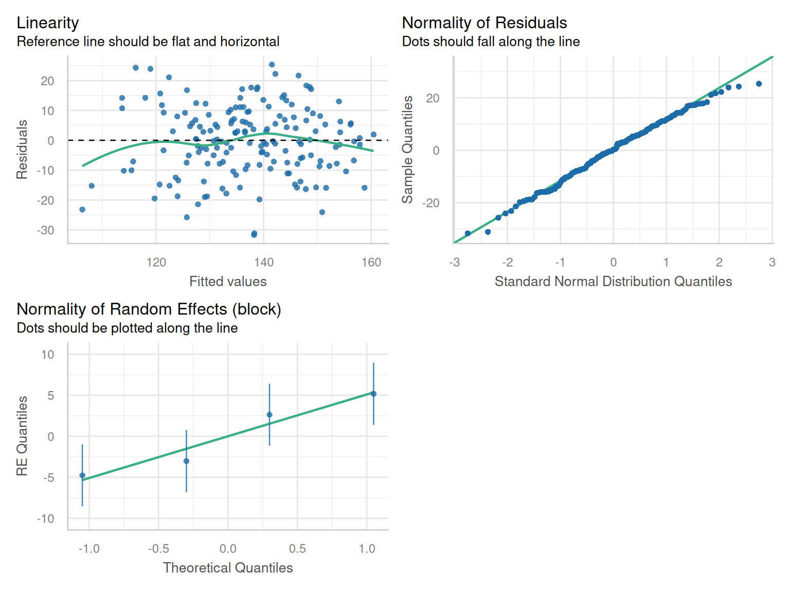
5.2.4 Inference
Estimates for each treatment level can be obtained with the ‘emmeans’ package.
Note
R syntax for estimating model marginal means is the same for lme4 and nlme.
rcbd_emm1 <- emmeans(model_rcbd_lmer, ~ variety)
as.data.frame(rcbd_emm1) |> arrange(desc(emmean)) |> head(n = 10)
variety emmean SE df lower.CL upper.CL
Rosalyn 155.2703 7.212203 77.85 140.9115 169.6292
IDO1005 153.5919 7.212203 77.85 139.2331 167.9508
OR2080641 152.6942 7.212203 77.85 138.3354 167.0530
Bobtail 151.6403 7.212203 77.85 137.2815 165.9992
UI Sparrow 151.6013 7.212203 77.85 137.2424 165.9601
Kaseberg 150.9768 7.212203 77.85 136.6179 165.3356
IDN-01-10704A 148.9861 7.212203 77.85 134.6273 163.3450
06-03303B 148.8300 7.212203 77.85 134.4712 163.1888
WB1529 148.2445 7.212203 77.85 133.8857 162.6034
DAS003 145.2000 7.212203 77.85 130.8412 159.5588
Degrees-of-freedom method: kenward-roger
Confidence level used: 0.95 rcbd_emm2 <- emmeans(model_rcbd_lme, ~ variety)
as.data.frame(rcbd_emm2) |> arrange(desc(emmean)) |> head(n = 10) variety emmean SE df lower.CL upper.CL
Rosalyn 155.2703 7.212203 3 132.3179 178.2228
IDO1005 153.5919 7.212203 3 130.6395 176.5444
OR2080641 152.6942 7.212203 3 129.7417 175.6466
Bobtail 151.6403 7.212203 3 128.6879 174.5928
UI Sparrow 151.6013 7.212203 3 128.6488 174.5537
Kaseberg 150.9768 7.212203 3 128.0243 173.9292
IDN-01-10704A 148.9861 7.212203 3 126.0337 171.9386
06-03303B 148.8300 7.212203 3 125.8775 171.7825
WB1529 148.2445 7.212203 3 125.2921 171.1970
DAS003 145.2000 7.212203 3 122.2476 168.1524
Degrees-of-freedom method: containment
Confidence level used: 0.95 These tables provide the estimated marginal means (“emmeans”), the standard error (“SE”) of those means, the degrees of freedom (“df”) and the lower and upper bounds of the 95% confidence interval (“lower.CL” and “upper.Cl”, respectively). As an additional step, the estimated marginal means were sorted from largest to smallest. Note the difference in degrees of freedom for each model. ‘lmerTest’ is implementing the Kenward-Roger’s method (Kuznetsova et al. 2017), while ‘nlme’ implements the containment method for degrees of freedom calculations. The Kenward-Roger’s method is preferred for small sample inference such as this example. Since it has a considerably larger estimate for the degrees of freedom, the resultant confidence intervals are much smaller compared to those using containment for df estimation.
At this point, the analysis goals have been met; we know the estimated means for each treatment and their rankings.
If you want to run ANOVA, it can be done quite easily. By default, sequential (type I) sums of squares is used by ‘nlme’, but partial (type 3) sums of squares is also possible. Containment is the only degrees of freedom calculation method enabled in ‘nlme’. The lmer-extender package ‘lmerTest’ implements SAS-like type 3 tests and the Kenward-Roger’s method for degrees of freedom approximation by default.1
1 The Type I method is called “sequential” sum of squares because it adds terms to the model one at a time; while type 3 (“partial”) drops model terms one at a time. This can effect the results of an F-test and p-value, but only when a data set is unbalanced across treatments, either due to design or missing data points. In this example, there is only one fixed effect (and the experiment is perfectly balanced), so the sums of squares choice is immaterial.
anova(model_rcbd_lmer, ddf = "Kenward-Roger")Type III Analysis of Variance Table with Kenward-Roger's method
Sum Sq Mean Sq NumDF DenDF F value Pr(>F)
variety 18354 447.65 41 123 2.4528 8.017e-05 ***
---
Signif. codes: 0 '***' 0.001 '**' 0.01 '*' 0.05 '.' 0.1 ' ' 1anova(model_rcbd_lme) numDF denDF F-value p-value
(Intercept) 1 123 2514.1283 <.0001
variety 41 123 2.4528 1e-04In this example, the difference in the degrees of freedom between models had little noticeable effect on downstream statistical contrasts or ANOVA.