library(dplyr)
library(lme4); library(lmerTest); library(broom.mixed)
library(emmeans); library(performance)8 Split-Split Plot Design
The concept of split-plot design can be extended to situations in which randomization restrictions may occur at any number of levels within the experiment. If there are two levels of randomization restriction, the layout is called a split-split plot design. The split-split plot design is an extension of the split-plot design to add a third level of treatment factor: one factor in the main plot, another in the split plot and a third factor in the split-split plot. The example shown below illustrates this experiment layout.
8.1 Details for split-split plot designs
The statistical model structure this design:
\[y_{ijk} = \mu + r_j + \alpha_i + \beta_k + (\alpha\beta)_{ik} + \gamma_n + (\alpha\gamma)_{in} + (\gamma\beta)_{nk} + (\alpha\beta\gamma)_{ikn} + \epsilon_{ijk} + \delta_{ijkn}\]
Where:
\(\mu\) = overall experimental mean
\(r\) = replication effect (random)
\(\alpha\) = main effect of whole plot (fixed)
\(\beta\) = main effect of split plot (fixed)
\(\gamma\) = main effect of split-split plot (fixed)
\(\epsilon_{ij}\) = whole plot error
\(\delta_{ijk}\) = split plot error
\(\tau_{xxx}\) = split-split plot error
The assumptions of the model includes normal distribution of both the error and the rep effects with a mean of zero and standard deviations of \(\sigma\) and \(\sigma_{sp}\), respectively.
\[\epsilon \sim N(0, \sigma_\epsilon)\]
\[\delta \sim N(0, \sigma_{sp})\]
\[\tau \sim N(0, \sigma_{ssp})\]
8.2 Example Analysis
library(dplyr)
library(nlme); library(emmeans)
library(broom.mixed); library(performance)
In this example, we have a rice yield data from the agricolae package (data set “ssp”). The experiment consists of 3 different rice varieties grown under 3 management practices and 5 nitrogen levels in the split-split plot design.
rice <- read.csv(here::here("data", "rice_ssp.csv"))| block | blocking unit |
| nitrogen | different nitrogen fertilizer rates as main plot with 5 levels |
| management | management practices as split plot with 3 levels |
| variety | crop variety being a split-split plot with 3 levels |
| yield | yield (bushels per acre) |
In this example, note that there are two randomization restrictions within each block: nitrogen & management. The order is which nitrogen treatments are applied is randomly selected. The 3 management practices are randomly assigned to the split plots. Finally, within a particular management, the 3 varieties are tested in a random order, forming 3 split-split plots.
8.2.1 Data integrity checks
Before analyzing the data let’s do some preliminary data quality checks.
- Check structure of the data
We will start with evaluation of the structure of the data where class of block, nitrogen, management and variety should be a character/factor and yield should be numeric.
str(rice)'data.frame': 135 obs. of 5 variables:
$ block : int 1 1 1 1 1 1 1 1 1 1 ...
$ nitrogen : int 0 0 0 50 50 50 80 80 80 110 ...
$ management: chr "m1" "m2" "m3" "m1" ...
$ variety : int 1 1 1 1 1 1 1 1 1 1 ...
$ yield : num 3.32 3.77 4.66 3.19 3.62 ...Here we need to convert block, nitrogen, variety, and management to data type character.
rice$block <- as.character(rice$block)
rice$nitrogen <- as.character(rice$nitrogen)
rice$management <- as.character(rice$management)
rice$variety <- as.character(rice$variety)- Inspect the independent variables
Next, run a cross tabulations to check balance of observations across independent variables:
table(rice$variety, rice$nitrogen, rice$management), , = m1
0 110 140 50 80
1 3 3 3 3 3
2 3 3 3 3 3
3 3 3 3 3 3
, , = m2
0 110 140 50 80
1 3 3 3 3 3
2 3 3 3 3 3
3 3 3 3 3 3
, , = m3
0 110 140 50 80
1 3 3 3 3 3
2 3 3 3 3 3
3 3 3 3 3 3It looks perfectly balanced, with exactly 3 observation per treatment group.
- Check the extent of missing data
colSums(is.na(rice)) block nitrogen management variety yield
0 0 0 0 0 Perfect! no missing values here.
- Inspect the dependent variable
Last, check the distribution of the dependent variable by plotting a histogram of yield values using hist() in R.
hist(rice$yield, main = NA, xlab = "yield")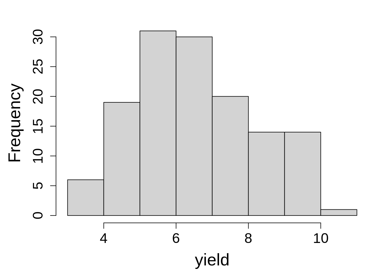
8.2.2 Model Building
The model and analysis of variance of a split-split plot design is comprised of three levels: the main plot, split plot, and split-split plot level. We will use the nesting notation in the random part because nitrogen and management are nested in blocks. We can do blocks as fixed or random.
model_lmer <- lmer(yield ~ nitrogen * management * variety + (1|block/nitrogen/management),
                   data = rice,
                   na.action = na.exclude)
boundary (singular) fit: see help('isSingular')tidy(model_lmer)# A tibble: 49 × 8
effect group term estimate std.error statistic df p.value
<chr> <chr> <chr> <dbl> <dbl> <dbl> <dbl> <dbl>
1 fixed <NA> (Intercept) 3.90 0.386 10.1 89.7 1.79e-16
2 fixed <NA> nitrogen110 0.753 0.545 1.38 89.7 1.71e- 1
3 fixed <NA> nitrogen140 0.165 0.545 0.302 89.7 7.63e- 1
4 fixed <NA> nitrogen50 0.335 0.545 0.614 89.7 5.41e- 1
5 fixed <NA> nitrogen80 1.33 0.545 2.44 89.7 1.68e- 2
6 fixed <NA> managementm2 0.420 0.540 0.779 80.0 4.38e- 1
7 fixed <NA> managementm3 1.43 0.540 2.65 80.0 9.82e- 3
8 fixed <NA> variety2 1.45 0.540 2.68 80.0 8.83e- 3
9 fixed <NA> variety3 1.48 0.540 2.74 80.0 7.49e- 3
10 fixed <NA> nitrogen110:managem… 0.377 0.763 0.493 80.0 6.23e- 1
# ℹ 39 more rowsmodel_lme <- lme(yield ~ nitrogen*management*variety,
random = ~ 1|block/nitrogen/management,
data = rice,
na.action = na.exclude)
tidy(model_lme)Warning in tidy.lme(model_lme): ran_pars not yet implemented for multiple
levels of nesting# A tibble: 45 × 7
effect term estimate std.error df statistic p.value
<chr> <chr> <dbl> <dbl> <dbl> <dbl> <dbl>
1 fixed (Intercept) 3.90 0.386 60 10.1 1.43e-14
2 fixed nitrogen110 0.753 0.545 8 1.38 2.05e- 1
3 fixed nitrogen140 0.165 0.545 8 0.302 7.70e- 1
4 fixed nitrogen50 0.335 0.545 8 0.614 5.56e- 1
5 fixed nitrogen80 1.33 0.545 8 2.44 4.08e- 2
6 fixed managementm2 0.420 0.540 20 0.779 4.45e- 1
7 fixed managementm3 1.43 0.540 20 2.65 1.55e- 2
8 fixed variety2 1.45 0.540 60 2.68 9.38e- 3
9 fixed variety3 1.48 0.540 60 2.74 7.99e- 3
10 fixed nitrogen110:managementm2 0.377 0.763 20 0.493 6.27e- 1
# ℹ 35 more rowsFor information on what boundary (singular) fit means, please refer to Chapter 14. For now, this warning message will be ignored.
8.2.3 Check Model Assumptions
check_model(model_lmer, check = c('qq', 'linearity', 'reqq'), detrend=FALSE, alpha = 0)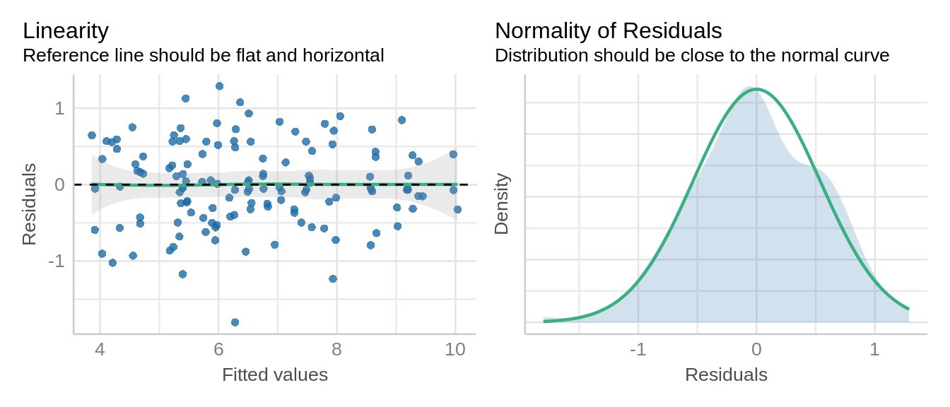
check_model(model_lme, check = c('qq', 'linearity'), detrend=FALSE)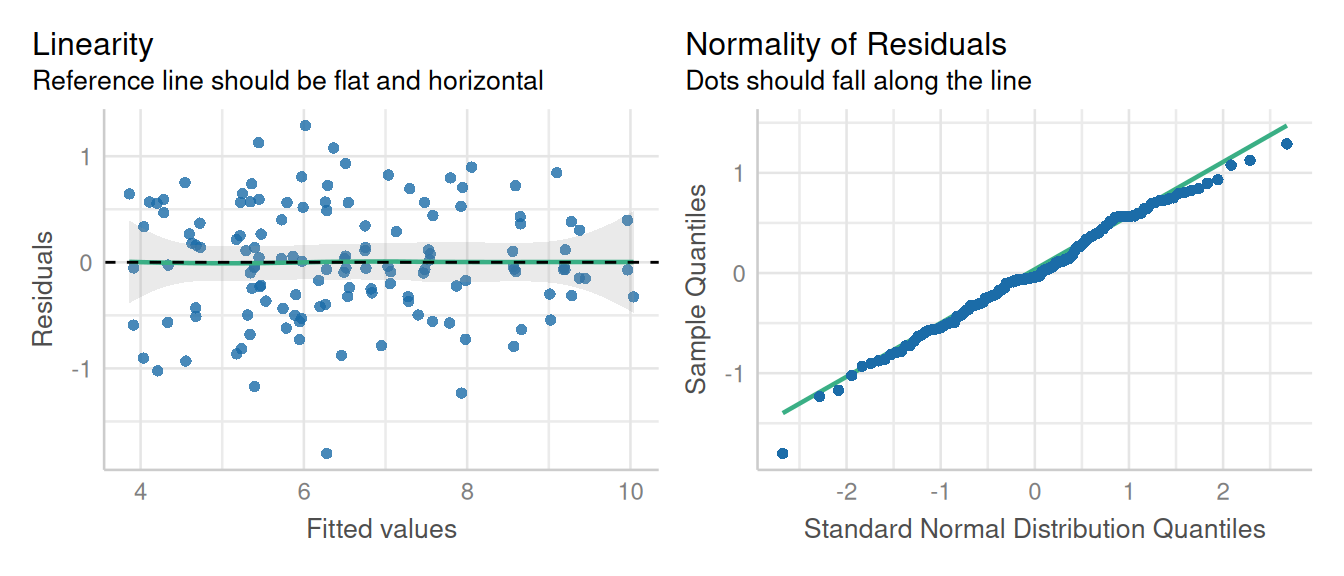
The assumptions of homescedascity and normality of residuals appear met.
8.2.4 Inference
Let’s look at the analysis of variance for fixed effects and their interaction effect on rice yield.
car::Anova(model_lmer, type = "III")Analysis of Deviance Table (Type III Wald chisquare tests)
Response: yield
Chisq Df Pr(>Chisq)
(Intercept) 102.1211 1 < 2.2e-16 ***
nitrogen 7.6641 4 0.104685
management 7.3923 2 0.024819 *
variety 9.8259 2 0.007351 **
nitrogen:management 1.6941 8 0.988997
nitrogen:variety 21.3448 8 0.006286 **
management:variety 8.8771 4 0.064245 .
nitrogen:management:variety 8.4629 16 0.933876
---
Signif. codes: 0 '***' 0.001 '**' 0.01 '*' 0.05 '.' 0.1 ' ' 1anova(model_lme, type = "marginal") numDF denDF F-value p-value
(Intercept) 1 60 102.12108 <.0001
nitrogen 4 8 1.91603 0.2012
management 2 20 3.69617 0.0431
variety 2 60 4.91295 0.0106
nitrogen:management 8 20 0.21177 0.9850
nitrogen:variety 8 60 2.66810 0.0141
management:variety 4 60 2.21929 0.0775
nitrogen:management:variety 16 60 0.52893 0.9210we observed a significant impact of management, variety, and nitrogen x variety interaction effect on rice yield.
Next, we can estimate the marginal means for each treatment factor (variety, nitrogen, management) which will be averaged across other factors and their interaction.
emmeans(model_lmer, ~ management)NOTE: Results may be misleading due to involvement in interactions management emmean SE df lower.CL upper.CL
m1 5.90 0.102 11.2 5.68 6.12
m2 6.49 0.102 11.2 6.26 6.71
m3 7.28 0.102 11.2 7.05 7.50
Results are averaged over the levels of: nitrogen, variety
Degrees-of-freedom method: kenward-roger
Confidence level used: 0.95 emmeans(model_lmer, ~ nitrogen*variety)NOTE: Results may be misleading due to involvement in interactions nitrogen variety emmean SE df lower.CL upper.CL
0 1 4.51 0.227 49 4.06 4.97
110 1 5.44 0.227 49 4.99 5.90
140 1 5.08 0.227 49 4.62 5.53
50 1 4.76 0.227 49 4.31 5.22
80 1 5.83 0.227 49 5.38 6.29
0 2 5.16 0.227 49 4.71 5.62
110 2 6.92 0.227 49 6.47 7.38
140 2 7.29 0.227 49 6.83 7.74
50 2 6.02 0.227 49 5.56 6.47
80 2 6.59 0.227 49 6.13 7.04
0 3 6.48 0.227 49 6.02 6.93
110 3 8.44 0.227 49 7.99 8.90
140 3 9.34 0.227 49 8.88 9.79
50 3 7.88 0.227 49 7.42 8.34
80 3 8.56 0.227 49 8.11 9.02
Results are averaged over the levels of: management
Degrees-of-freedom method: kenward-roger
Confidence level used: 0.95 emmeans(model_lme, ~ management)NOTE: Results may be misleading due to involvement in interactions management emmean SE df lower.CL upper.CL
m1 5.90 0.102 2 5.46 6.34
m2 6.49 0.102 2 6.05 6.92
m3 7.28 0.102 2 6.84 7.71
Results are averaged over the levels of: nitrogen, variety
Degrees-of-freedom method: containment
Confidence level used: 0.95 emmeans(model_lme, ~ nitrogen*variety)NOTE: Results may be misleading due to involvement in interactions nitrogen variety emmean SE df lower.CL upper.CL
0 1 4.51 0.227 2 3.54 5.49
110 1 5.44 0.227 2 4.47 6.42
140 1 5.08 0.227 2 4.10 6.05
50 1 4.76 0.227 2 3.79 5.74
80 1 5.83 0.227 2 4.86 6.81
0 2 5.16 0.227 2 4.19 6.14
110 2 6.92 0.227 2 5.95 7.90
140 2 7.29 0.227 2 6.31 8.27
50 2 6.02 0.227 2 5.04 6.99
80 2 6.59 0.227 2 5.61 7.57
0 3 6.48 0.227 2 5.50 7.46
110 3 8.44 0.227 2 7.47 9.42
140 3 9.34 0.227 2 8.36 10.31
50 3 7.88 0.227 2 6.90 8.86
80 3 8.56 0.227 2 7.59 9.54
Results are averaged over the levels of: management
Degrees-of-freedom method: containment
Confidence level used: 0.95 Notice we get a message that the estimated means for ‘nitrogen x variety’ are averaged over the levels of ‘management’. So we need to be careful about this while making conslusions/recommendations.
Nested random effects
You may have noticed the order of random effects in model statement:
model_lme <- lme(yield ~ nitrogen*management*variety,
                  random = ~ 1|block/nitrogen/management,
                  data = rice,
                  na.action = na.exclude)
The random effects follow the order of ~1|block/main plot/split-plot. While fitting the model for split-split plot design please make sure to have a clear understanding of the main plot, split-plot and split-split plot factors to avoid having an erroneous model.