Section 6 RCBD Example: SAS

6.1 Load and Explore Data

These data are from a winter wheat variety trial in Alliance, Nebraska (Stroup, Baenziger, and Mulitze 1994) and are commonly used to demonstrate spatial adjustment in linear modeling. The data represent yields of 56 varieties originally laid out in a randomized complete block design (RCB). The local topography combined with winter kill, however, induced spatial variability that did not correspond to the RCB design (Stroup 2013) which produced biased estimates in a standard unadjusted analysis.

The code below reads the data from a CSV file located the GitHub repo for this book. The data file can be downloaded from here. In this file, missing values for yield are denoted as ‘NA’. These values are not actually missing, but represent blank plots separating blocks in the original design of the study. The PROC FORMAT section converts these to numeric missing values in SAS (defined as a single period). They are then removed from the data before proceeding to analyses. Also note that row and column indices are multiplied by constants to convert them to the meter dimensions of the plots. .

The first six observations are displayed. The data contains variables for variety (gen), replication (rep), yield, and column and row identifiers.

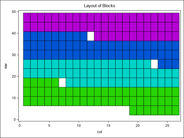
Last, a map of the 4 replications (blocks) from the original experimental design is shown.

proc format;
  invalue has_NA
  'NA' = .;
;

filename NIN url "https://raw.githubusercontent.com/IdahoAgStats/guide-to-field-trial-spatial-analysis/master/data/stroup_nin_wheat.csv";

data alliance;
    infile NIN firstobs=2 delimiter=',';
    informat yield has_NA.;
    input entry $   rep $   yield   col row;
    Row  = 4.3*Row;
    Col = 1.2*Col;
    if yield=. then delete;
run;

proc print data=alliance(obs=6);
title1 ' Alliance Nebraska Wheat Variety Data';

run;
ODS html GPATH = ".\img\" ;

proc sgplot data=alliance;
    styleattrs datacolors=(cx28D400 cx00D4C8 cx0055D4 cxB400D4) datalinepatterns=(solid dash);
    HEATMAPPARM y=row x=col COLORgroup=rep/ outline; 
title1 'Layout of Blocks';
run;

Alliance Nebraska Wheat Variety Data

Obs	yield	entry	rep	col	row
1	29.25	Lancer	R1	19.2	4.3
2	31.55	Brule	R1	20.4	4.3
3	35.05	Redland	R1	21.6	4.3
4	30.10	Cody	R1	22.8	4.3
5	33.05	Arapahoe	R1	24.0	4.3
6	30.25	NE83404	R1	25.2	4.3

The SGPlot Procedure

6.1.1 Plots of Field Trends

A first step in assessing spatial variability is to plot the data to visually assess any trends or patterns. This code uses the SGPLOT procedure to examine spatial patterns through a heat map of yields, as well as potential trends across replications, columns, and rows using box plots.

ODS html GPATH = ".\img\" ;

proc sgplot data=alliance;
    HEATMAPPARM y=Row x=Col COLORRESPONSE=yield/ colormodel=(blue yellow green); 
run;

proc sgplot data=alliance;
    vbox yield/category=rep FILLATTRS=(color=red) LINEATTRS=(color=black) WHISKERATTRS=(color=black);
run;

proc sgplot data=alliance;
    vbox yield/category=Col FILLATTRS=(color=yellow) LINEATTRS=(color=black) WHISKERATTRS=(color=black);
run;

proc sgplot data=alliance;
    vbox yield/category=Row FILLATTRS=(color=blue) LINEATTRS=(color=black) WHISKERATTRS=(color=black);
run;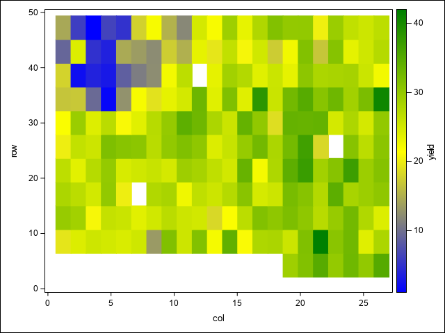

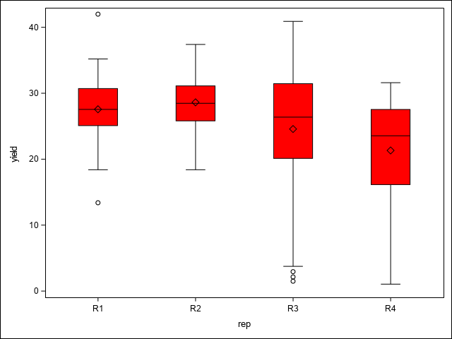
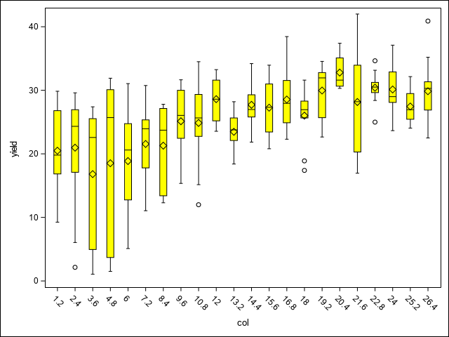
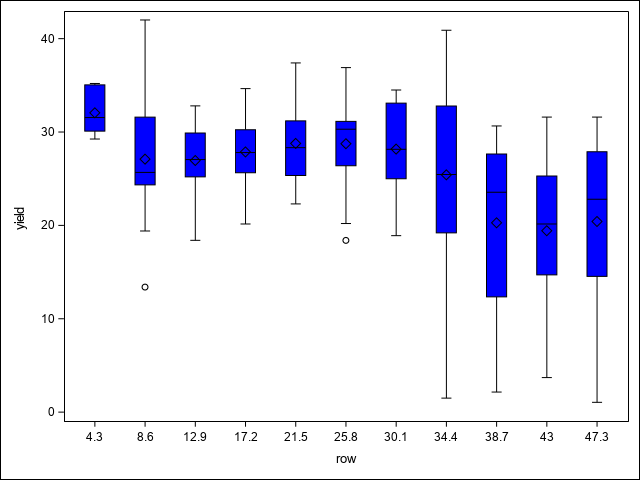
The SGPlot Procedure

In the heat map, there is a notable region where yield dips in the north west corner of the study area. This area runs across the two top most blocks and is positioned towards their ends, making those blocks non-homogeneous. As Stroup (Stroup 2013) notes, this is due to a hilly area with low snow cover and high exposure to low winter temperatures. The box plots demonstrate this pattern across blocks, columns, and rows as well. From these initial graphics, it is clear there are discernible spatial patterns and trends present.

6.2 Estimating and Testing Spatial Correlation

6.2.1 Examine the Number of Distance Pairs and Maximum Lags between Residuals

The process of modeling spatial variability begins by obtaining the residuals from the original RCB analysis. Here PROC MIXED is used to fit the RCB model and output the model residuals to the SAS data set “residuals”.


ods html close;
proc mixed data=alliance;
   class Rep Entry;
   model Yield = Entry / outp=residuals;
   random Rep;
run;
ods html;

Examining and estimating spatial variability typically proceeds in several steps. In SAS, these can all be accomplished using PROC VARIOGRAM. In this first step, we summarize the potential distances (lags) between row/column positions. The nhclasses option sets a value for the number of lag classes or bins to try. Some trial and error here may be necessary in order to find a good setting, however, this value should be big enough to cover the range of possible distances between data row and column coordinates. Setting this initially to 40 was found to be a reasonable choice here. The novariogram option tells SAS to only look at these distances and not compute the empirical semivariance values yet.


/* Examine lag distance & maxlag */
ODS html GPATH = ".\img\" ;

proc variogram data=residuals;
   compute novariogram nhclasses=40;
   coordinates xc=row yc=col;
   var resid;
run;

Dependent Variable: Resid

Number of Observations Read	224
Number of Observations Used	224

Spatial Distribution of Resid Observations

Pairs Information
Number of Lags	41
Lag Distance	1.25
Maximum Data Distance in row	43.00
Maximum Data Distance in col	25.20
Maximum Data Distance	49.84

Pairwise Distance Intervals
Lag Class	Bounds		Number of Pairs	Percentage of Pairs
0	0.00	0.62	0	0.00%
1	0.62	1.87	210	0.84%
2	1.87	3.12	199	0.80%
3	3.12	4.36	387	1.55%
4	4.36	5.61	917	3.67%
5	5.61	6.85	832	3.33%
6	6.85	8.10	462	1.85%
7	8.10	9.35	1571	6.29%
8	9.35	10.59	1215	4.86%
9	10.59	11.84	615	2.46%
10	11.84	13.08	1252	5.01%
11	13.08	14.33	1563	6.26%
12	14.33	15.58	910	3.64%
13	15.58	16.82	867	3.47%
14	16.82	18.07	1805	7.23%
15	18.07	19.31	1058	4.24%
16	19.31	20.56	873	3.50%
17	20.56	21.81	1352	5.41%
18	21.81	23.05	935	3.74%
19	23.05	24.30	943	3.78%
20	24.30	25.54	517	2.07%
21	25.54	26.79	1439	5.76%
22	26.79	28.04	513	2.05%
23	28.04	29.28	387	1.55%
24	29.28	30.53	868	3.48%
25	30.53	31.77	555	2.22%
26	31.77	33.02	350	1.40%
27	33.02	34.27	172	0.69%
28	34.27	35.51	770	3.08%
29	35.51	36.76	259	1.04%
30	36.76	38.00	188	0.75%
31	38.00	39.25	362	1.45%
32	39.25	40.50	207	0.83%
33	40.50	41.74	147	0.59%
34	41.74	42.99	59	0.24%
35	42.99	44.23	117	0.47%
36	44.23	45.48	49	0.20%
37	45.48	46.73	30	0.12%
38	46.73	47.97	11	0.04%
39	47.97	49.22	7	0.03%
40	49.22	50.46	3	0.01%

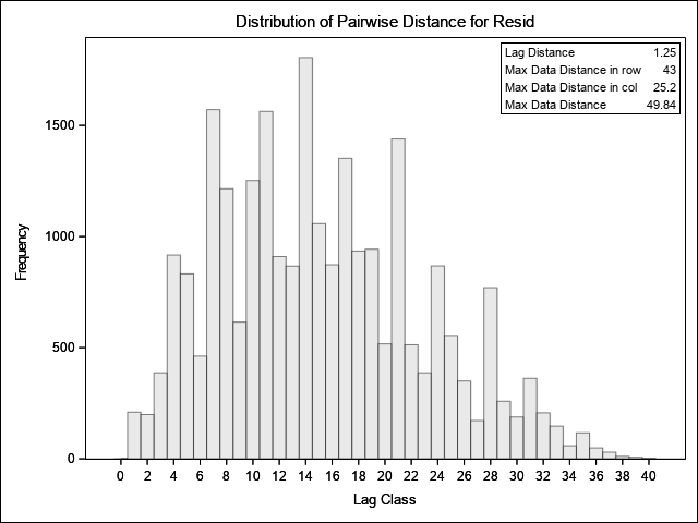
Distribution of Pairwise Distance for Resid

This output indicates that, with 40 bins, the minimum lag distance is approximately 1.2m and that the maximum lag distances vary from 25 to 43m in rows and columns, respectively. The histogram graphically displays the number of pairs at each lag distance bin. Ideally, we want bins that have at least 30 pairs to improve accuracy in estimation of the empirical semivariance. There is sufficient data here such that setting the maximum lag to 30 results in bins that have much more than 30 pairs and will provide an accurate estimate of semivariance.

6.2.2 Compute Moran’s I and Geary’s C.

Two common metrics of spatial correlation are Moran’s I and Geary’s c. Both these measures are essentially weighted correlations between pairs of observations and measure global and local variability, respectively. If no spatial correlation is present, Moran’s I has an expected value close to 0.0 while Geary’s C will be close to 1.0. The estimates for I and C can be computed and tested against these null values with the PROC VARIOGRAM code below.

ODS html GPATH = ".\img\" ;

proc variogram data=residuals plots(only)=moran ;
   compute lagd=1.2 maxlag=30 novariogram autocorr(assum=nor) ;
   coordinates xc=row yc=col;
   var resid;
run;

Dependent Variable: Resid

Number of Observations Read	224
Number of Observations Used	224

Pairs Information
Number of Lags	11
Lag Distance	4.98
Maximum Data Distance in row	43.00
Maximum Data Distance in col	25.20
Maximum Data Distance	49.84

Pairwise Distance Intervals
Lag Class	Bounds		Number of Pairs	Percentage of Pairs
0	0.00	2.49	409	1.64%
1	2.49	7.48	2598	10.40%
2	7.48	12.46	3757	15.04%
3	12.46	17.44	5204	20.84%
4	17.44	22.43	4738	18.97%
5	22.43	27.41	3455	13.83%
6	27.41	32.40	2241	8.97%
7	32.40	37.38	1518	6.08%
8	37.38	42.36	813	3.26%
9	42.36	47.35	228	0.91%
10	47.35	52.33	15	0.06%

Autocorrelation Statistics
Assumption	Coefficient	Observed	Expected	Std Dev	Z	Pr > \|Z\|
Normality	Moran's I	0.330	-0.00495	0.0836	4.01	<.0001
Normality	Geary's c	0.614	1.00000	0.0901	-4.29	<.0001

Moran Scatter Plot for Resid

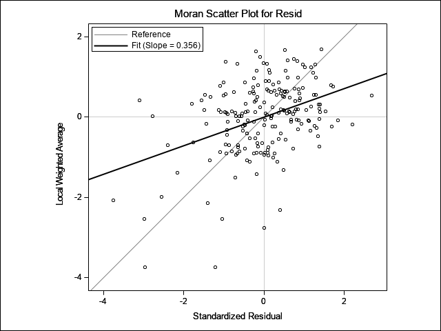
Both Moran’s I and Geary’s C are significant here, indicating the presence of spatial correlation. The accompanying scatter plot of residuals vs lag distance also show a positive correlation where residuals increase in magnitude with increasing distance between points.

6.3 Estimation and Modeling of Semivariance

6.3.1 Estimating Empirical Semivariance

Using the lag distance and maximum lag values obtained in the previous steps, we can now use the compute statement to estimate an empirical variogram as described in Section 2

ODS html GPATH = ".\img\" ;

proc variogram data=residuals plots(only)=(semivar);
   coordinates xc=Col yc=Row;
   compute lagd=1.2 maxlags=30;
  var resid;
run;

Dependent Variable: Resid

Number of Observations Read	224
Number of Observations Used	224

Dependent Variable: Resid

Empirical Semivariogram
Lag Class	Pair Count	Average Distance	Semivariance
0	0	.	.
1	210	1.20	20.133
2	199	2.40	22.159
3	188	3.60	24.453
4	1116	4.64	21.737
5	832	6.01	25.005
6	462	7.32	28.096
7	1268	8.63	26.521
8	996	9.54	30.424
9	904	10.75	34.523
10	589	11.86	37.983
11	1812	13.14	32.064
12	1164	14.30	36.624
13	1021	15.67	41.839
14	1207	17.12	38.201
15	1329	17.97	38.456
16	988	19.19	41.319
17	691	20.46	47.746
18	1556	21.69	39.750
19	965	22.82	41.013
20	558	23.98	42.051
21	522	25.13	43.919
22	1273	26.21	35.351
23	588	27.55	42.812
24	312	28.69	43.350
25	868	30.13	37.531
26	555	31.11	42.186
27	350	32.41	48.901
28	172	33.60	56.251
29	704	34.68	33.781
30	325	35.91	45.543

Dependent Variable: Resid

Empirical Semivariogram Plot for Resid

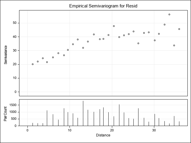
In the plot, the semi-variance increases as distance between points increases up to approximately 20m where it begins to level off. This type of pattern is very common for spatial relationships.

6.3.2 Fitting an Empirical Variogram Model

In Section 3, several theoretical variogram models were described. We can use PROC VARIOGRAM to fit and compare any number of these models. In the code below, the Gaussian, Exponential, Power, and Spherical models are fit using the model statement. By default when several models are listed, SAS will carry out a more sophisticated spatial modeling approach that uses combinations of these models. We, however, just want to focus on single model scenarios. Hence, the nest=1 option is given which restricts the variogram modeling to single models only.

ODS html GPATH = ".\img\" ;

proc variogram data=residuals plots(only)=(fitplot);
   coordinates xc=Col yc=Row;
   compute lagd=1.2 maxlags=30;
   model form=auto(mlist=(gau, exp, pow, sph) nest=1);
  var resid;
run;

Dependent Variable: Resid

Number of Observations Read	224
Number of Observations Used	224

Dependent Variable: Resid

Empirical Semivariogram
Lag Class	Pair Count	Average Distance	Semivariance
0	0	.	.
1	210	1.20	20.133
2	199	2.40	22.159
3	188	3.60	24.453
4	1116	4.64	21.737
5	832	6.01	25.005
6	462	7.32	28.096
7	1268	8.63	26.521
8	996	9.54	30.424
9	904	10.75	34.523
10	589	11.86	37.983
11	1812	13.14	32.064
12	1164	14.30	36.624
13	1021	15.67	41.839
14	1207	17.12	38.201
15	1329	17.97	38.456
16	988	19.19	41.319
17	691	20.46	47.746
18	1556	21.69	39.750
19	965	22.82	41.013
20	558	23.98	42.051
21	522	25.13	43.919
22	1273	26.21	35.351
23	588	27.55	42.812
24	312	28.69	43.350
25	868	30.13	37.531
26	555	31.11	42.186
27	350	32.41	48.901
28	172	33.60	56.251
29	704	34.68	33.781
30	325	35.91	45.543

Dependent Variable: Resid

Angle: Omnidirectional

Semivariogram Model Fitting
Model	Selection from 4 form combinations

Fit Summary
Class	Model	Weighted SSE	AIC
1	Gau	90.90699	39.25919
2	Sph	95.41630	40.71156
3	Exp	111.51151	45.38791
4	Pow	131.80037	50.40273

Semivariogram Model Fitting
Name	Gaussian
Label	Gau

Model Information
Parameter	Initial Value
Nugget	18.1070
Scale	27.0845
Range	17.9554

Optimization Information
Optimization Technique	Dual Quasi-Newton
Parameters in Optimization	3
Lower Boundaries	3
Upper Boundaries	0
Starting Values From	PROC

Parameter Estimates
Parameter	Estimate	Approx Std Error	DF	t Value	Approx Pr > \|t\|
Nugget	19.6331	0.5918	27	33.18	<.0001
Scale	22.0523	0.6610	27	33.36	<.0001
Range	11.6661	0.4488	27	26.00	<.0001

Dependent Variable: Resid

WLS Fitted Semivariograms Plot for Resid

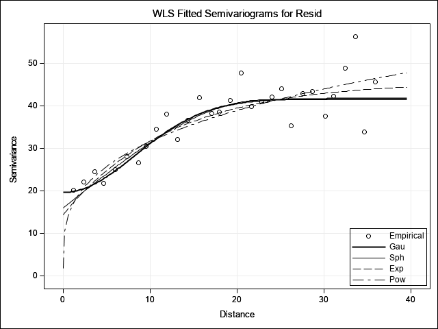
The table Fit Summary provides statistics on each variogram model fit. The AIC or SSE statistics can be used as a guide for model selection where smaller values indicate a better fit. For this data, the Gaussian model is rated as “best”, although the Spherical model is relatively similar. Given the numerically lower AIC and SSE values, however, PROC VARIOGRAM selects the Gaussian model and reports those semivariogram model parameter estimates in the final table. These parameter estimates will be used in the next step. The plot shown at the end provides a visual comparison each variogram model fit with the selected Gaussian model highlighted in bold.

6.4 Using the Estimated variogram in an Adjusted Analysis

The previous steps have:
1. Diagnosed the presence and pattern of spatial variability.
2. Identified and estimated the a model to describe the variability

The last step is to utilize this information in a statistical analysis as outlined at the beginning of Section 3. To do this, the linear mixed model procedure PROC MIXED will be used to incorporate the spatial variability into the linear model variance-covariance matrix, assuming the variogram model identified above.

As an initial step, for comparison purposes, the unadjusted RCB model is run first and the means saved in data set “NIN_RCBD_means”.

6.4.1 Unadjusted RCBD Model


/** Fit unadjusted RCBD model **/
ODS html GPATH = ".\img\" ;

proc mixed data=alliance ;
    class entry rep;
    model yield = entry ;
    random rep;
    lsmeans entry/cl;
    ods output LSMeans=NIN_RCBD_means;
    title1 'NIN data: RCBD';
run;

NIN data: RCBD

Model Information
Data Set	WORK.ALLIANCE
Dependent Variable	yield
Covariance Structure	Variance Components
Estimation Method	REML
Residual Variance Method	Profile
Fixed Effects SE Method	Model-Based
Degrees of Freedom Method	Containment

Class Level Information
Class	Levels	Values
entry	56	Arapahoe Brule Buckskin Centura Centurk7 Cheyenne Cody Colt Gage Homestea KS831374 Lancer Lancota NE83404 NE83406 NE83407 NE83432 NE83498 NE83T12 NE84557 NE85556 NE85623 NE86482 NE86501 NE86503 NE86507 NE86509 NE86527 NE86582 NE86606 NE86607 NE86T666 NE87403 NE87408 NE87409 NE87446 NE87451 NE87457 NE87463 NE87499 NE87512 NE87513 NE87522 NE87612 NE87613 NE87615 NE87619 NE87627 Norkan Redland Roughrid Scout66 Siouxlan TAM107 TAM200 Vona
rep	4	R1 R2 R3 R4

Dimensions
Covariance Parameters	2
Columns in X	57
Columns in Z	4
Subjects	1
Max Obs per Subject	224

Number of Observations
Number of Observations Read	224
Number of Observations Used	224
Number of Observations Not Used	0

Iteration History
Iteration	Evaluations	-2 Res Log Like	Criterion
0	1	1240.74178756
1	1	1217.70153249	0.00000000

Convergence criteria met.

Covariance Parameter Estimates
Cov Parm	Estimate
rep	9.8829
Residual	49.5824

Fit Statistics
-2 Res Log Likelihood	1217.7
AIC (Smaller is Better)	1221.7
AICC (Smaller is Better)	1221.8
BIC (Smaller is Better)	1220.5

Type 3 Tests of Fixed Effects
Effect	Num DF	Den DF	F Value	Pr > F
entry	55	165	0.88	0.7119

Least Squares Means
Effect	entry	Estimate	Standard Error	DF	t Value	Pr > \|t\|	Alpha	Lower	Upper
entry	Arapahoe	29.4375	3.8557	165	7.63	<.0001	0.05	21.8247	37.0503
entry	Brule	26.0750	3.8557	165	6.76	<.0001	0.05	18.4622	33.6878
entry	Buckskin	25.5625	3.8557	165	6.63	<.0001	0.05	17.9497	33.1753
entry	Centura	21.6500	3.8557	165	5.62	<.0001	0.05	14.0372	29.2628
entry	Centurk7	30.3000	3.8557	165	7.86	<.0001	0.05	22.6872	37.9128
entry	Cheyenne	28.0625	3.8557	165	7.28	<.0001	0.05	20.4497	35.6753
entry	Cody	21.2125	3.8557	165	5.50	<.0001	0.05	13.5997	28.8253
entry	Colt	27.0000	3.8557	165	7.00	<.0001	0.05	19.3872	34.6128
entry	Gage	24.5125	3.8557	165	6.36	<.0001	0.05	16.8997	32.1253
entry	Homestea	27.6375	3.8557	165	7.17	<.0001	0.05	20.0247	35.2503
entry	KS831374	24.1250	3.8557	165	6.26	<.0001	0.05	16.5122	31.7378
entry	Lancer	28.5625	3.8557	165	7.41	<.0001	0.05	20.9497	36.1753
entry	Lancota	26.5500	3.8557	165	6.89	<.0001	0.05	18.9372	34.1628
entry	NE83404	27.3875	3.8557	165	7.10	<.0001	0.05	19.7747	35.0003
entry	NE83406	24.2750	3.8557	165	6.30	<.0001	0.05	16.6622	31.8878
entry	NE83407	22.6875	3.8557	165	5.88	<.0001	0.05	15.0747	30.3003
entry	NE83432	19.7250	3.8557	165	5.12	<.0001	0.05	12.1122	27.3378
entry	NE83498	30.1250	3.8557	165	7.81	<.0001	0.05	22.5122	37.7378
entry	NE83T12	21.5625	3.8557	165	5.59	<.0001	0.05	13.9497	29.1753
entry	NE84557	20.5250	3.8557	165	5.32	<.0001	0.05	12.9122	28.1378
entry	NE85556	26.3875	3.8557	165	6.84	<.0001	0.05	18.7747	34.0003
entry	NE85623	21.7250	3.8557	165	5.63	<.0001	0.05	14.1122	29.3378
entry	NE86482	24.2875	3.8557	165	6.30	<.0001	0.05	16.6747	31.9003
entry	NE86501	30.9375	3.8557	165	8.02	<.0001	0.05	23.3247	38.5503
entry	NE86503	32.6500	3.8557	165	8.47	<.0001	0.05	25.0372	40.2628
entry	NE86507	23.7875	3.8557	165	6.17	<.0001	0.05	16.1747	31.4003
entry	NE86509	26.8500	3.8557	165	6.96	<.0001	0.05	19.2372	34.4628
entry	NE86527	22.0125	3.8557	165	5.71	<.0001	0.05	14.3997	29.6253
entry	NE86582	24.5375	3.8557	165	6.36	<.0001	0.05	16.9247	32.1503
entry	NE86606	29.7625	3.8557	165	7.72	<.0001	0.05	22.1497	37.3753
entry	NE86607	29.3250	3.8557	165	7.61	<.0001	0.05	21.7122	36.9378
entry	NE86T666	21.5375	3.8557	165	5.59	<.0001	0.05	13.9247	29.1503
entry	NE87403	25.1250	3.8557	165	6.52	<.0001	0.05	17.5122	32.7378
entry	NE87408	26.3000	3.8557	165	6.82	<.0001	0.05	18.6872	33.9128
entry	NE87409	21.3750	3.8557	165	5.54	<.0001	0.05	13.7622	28.9878
entry	NE87446	27.6750	3.8557	165	7.18	<.0001	0.05	20.0622	35.2878
entry	NE87451	24.6125	3.8557	165	6.38	<.0001	0.05	16.9997	32.2253
entry	NE87457	23.9125	3.8557	165	6.20	<.0001	0.05	16.2997	31.5253
entry	NE87463	25.9125	3.8557	165	6.72	<.0001	0.05	18.2997	33.5253
entry	NE87499	20.4125	3.8557	165	5.29	<.0001	0.05	12.7997	28.0253
entry	NE87512	23.2500	3.8557	165	6.03	<.0001	0.05	15.6372	30.8628
entry	NE87513	26.8125	3.8557	165	6.95	<.0001	0.05	19.1997	34.4253
entry	NE87522	25.0000	3.8557	165	6.48	<.0001	0.05	17.3872	32.6128
entry	NE87612	21.8000	3.8557	165	5.65	<.0001	0.05	14.1872	29.4128
entry	NE87613	29.4000	3.8557	165	7.63	<.0001	0.05	21.7872	37.0128
entry	NE87615	25.6875	3.8557	165	6.66	<.0001	0.05	18.0747	33.3003
entry	NE87619	31.2625	3.8557	165	8.11	<.0001	0.05	23.6497	38.8753
entry	NE87627	23.2250	3.8557	165	6.02	<.0001	0.05	15.6122	30.8378
entry	Norkan	24.4125	3.8557	165	6.33	<.0001	0.05	16.7997	32.0253
entry	Redland	30.5000	3.8557	165	7.91	<.0001	0.05	22.8872	38.1128
entry	Roughrid	21.1875	3.8557	165	5.50	<.0001	0.05	13.5747	28.8003
entry	Scout66	27.5250	3.8557	165	7.14	<.0001	0.05	19.9122	35.1378
entry	Siouxlan	30.1125	3.8557	165	7.81	<.0001	0.05	22.4997	37.7253
entry	TAM107	28.4000	3.8557	165	7.37	<.0001	0.05	20.7872	36.0128
entry	TAM200	21.2375	3.8557	165	5.51	<.0001	0.05	13.6247	28.8503
entry	Vona	23.6000	3.8557	165	6.12	<.0001	0.05	15.9872	31.2128

The F-statistic and accompanying large p-value for ‘gen’ indicate no differences between cultivars. This is surprising for a variety trial. The fit statistics (e.g. AIC) are helpful for model comparison, although on their own, these metrics do not have much meaning. The AIC value for this standard RCB analysis is 1221.7; let’s compare that number to that for the spatially-adjusted models (in the case of AIC, smaller numbers indicate a better fitting model). Another point of comparison is the standard error of the means: 3.8557.

The next step is to try a spatially-adjusted model. This is done by adding a repeated statement specifying the spatial model form (Gaussian, type=sp(gau)) and the variables related to spatial positions in the study (row, col). The local option tells SAS to use a nugget parameter in the Gaussian variogram model. The second additional statement is parms. This gives SAS a starting place for estimating the range, sill, and nugget parameters. The values given here are taken from the PROC VARIOGRAM output above. While this step can be omitted, it is recommended not to do so because, on its own, PROC MIXED can often have trouble narrowing in on reasonable parameter estimates. One reason for the preceding variogram steps was to obtain these parameter values so PROC MIXED has a good starting place for estimation. As before, the estimated means (adjusted now) are saved, this time in data set “NIN_Spatial_means”.

6.4.2 RCB Model with Spatial Covariance


/** Fit Gaussian adjusted model **/
/** Parms statement order: Range, Sill, Nugget **/
/** Model option "local" forces nugget into model **/
ODS html GPATH = ".\img\" ;

proc mixed data=alliance maxiter=150;
    class entry;
    model yield = entry /ddfm=kr;
    repeated/subject=intercept type=sp(gau) (Row Col) local;
    parms (11) (22) (19);
    lsmeans entry/cl;
    ods output LSMeans=NIN_Spatial_means;
    title1 'NIN data: Gaussian Spatial Adjustment';
run;

NIN data: Gaussian Spatial Adjustment

Model Information
Data Set	WORK.ALLIANCE
Dependent Variable	yield
Covariance Structure	Spatial Gaussian
Subject Effect	Intercept
Estimation Method	REML
Residual Variance Method	Profile
Fixed Effects SE Method	Kenward-Roger
Degrees of Freedom Method	Kenward-Roger

Class Level Information
Class	Levels	Values
entry	56	Arapahoe Brule Buckskin Centura Centurk7 Cheyenne Cody Colt Gage Homestea KS831374 Lancer Lancota NE83404 NE83406 NE83407 NE83432 NE83498 NE83T12 NE84557 NE85556 NE85623 NE86482 NE86501 NE86503 NE86507 NE86509 NE86527 NE86582 NE86606 NE86607 NE86T666 NE87403 NE87408 NE87409 NE87446 NE87451 NE87457 NE87463 NE87499 NE87512 NE87513 NE87522 NE87612 NE87613 NE87615 NE87619 NE87627 Norkan Redland Roughrid Scout66 Siouxlan TAM107 TAM200 Vona

Dimensions
Covariance Parameters	3
Columns in X	57
Columns in Z	0
Subjects	1
Max Obs per Subject	224

Number of Observations
Number of Observations Read	224
Number of Observations Used	224
Number of Observations Not Used	0

Parameter Search
CovP1	CovP2	CovP3	Variance	Res Log Like	-2 Res Log Like
11.0000	22.0000	19.0000	25.3339	-555.0999	1110.1998

Iteration History
Iteration	Evaluations	-2 Res Log Like	Criterion
1	2	1098.19938899	0.55691103
2	2	1073.55589724	0.01698755
3	2	1070.40479989	0.00621291
4	1	1067.58247826	0.00103523
5	1	1067.13250829	0.00007623
6	1	1067.10196425	0.00000066
7	1	1067.10171375	0.00000000

Convergence criteria met.

Covariance Parameter Estimates
Cov Parm	Subject	Estimate
Variance	Intercept	43.3874
SP(GAU)	Intercept	10.7004
Residual		15.3580

Fit Statistics
-2 Res Log Likelihood	1067.1
AIC (Smaller is Better)	1073.1
AICC (Smaller is Better)	1073.2
BIC (Smaller is Better)	1082.5

PARMS Model Likelihood Ratio Test
DF	Chi-Square	Pr > ChiSq
2	43.10	<.0001

Type 3 Tests of Fixed Effects
Effect	Num DF	Den DF	F Value	Pr > F
entry	55	136	1.84	0.0024

Least Squares Means
Effect	entry	Estimate	Standard Error	DF	t Value	Pr > \|t\|	Alpha	Lower	Upper
entry	Arapahoe	27.0657	3.2760	18.5	8.26	<.0001	0.05	20.1964	33.9351
entry	Brule	27.0363	3.2912	18.3	8.21	<.0001	0.05	20.1295	33.9430
entry	Buckskin	35.6362	3.3341	19.5	10.69	<.0001	0.05	28.6692	42.6032
entry	Centura	25.4196	3.2861	17.9	7.74	<.0001	0.05	18.5131	32.3261
entry	Centurk7	27.2432	3.2915	18.2	8.28	<.0001	0.05	20.3345	34.1519
entry	Cheyenne	25.0592	3.2843	18.3	7.63	<.0001	0.05	18.1660	31.9524
entry	Cody	24.0971	3.2733	18.5	7.36	<.0001	0.05	17.2346	30.9596
entry	Colt	25.7772	3.3473	18.5	7.70	<.0001	0.05	18.7570	32.7974
entry	Gage	25.0110	3.2920	18	7.60	<.0001	0.05	18.0941	31.9279
entry	Homestea	22.1425	3.2711	19.1	6.77	<.0001	0.05	15.2994	28.9856
entry	KS831374	26.9109	3.2537	18.8	8.27	<.0001	0.05	20.0954	33.7263
entry	Lancer	23.6478	3.2891	18.2	7.19	<.0001	0.05	16.7428	30.5528
entry	Lancota	21.7590	3.3014	18.5	6.59	<.0001	0.05	14.8367	28.6814
entry	NE83404	25.4502	3.2997	18.4	7.71	<.0001	0.05	18.5282	32.3721
entry	NE83406	26.5136	3.2808	18.5	8.08	<.0001	0.05	19.6355	33.3918
entry	NE83407	26.0105	3.3019	19.7	7.88	<.0001	0.05	19.1168	32.9041
entry	NE83432	22.3448	3.2852	18.3	6.80	<.0001	0.05	15.4503	29.2394
entry	NE83498	29.7725	3.3042	18.3	9.01	<.0001	0.05	22.8396	36.7055
entry	NE83T12	21.9692	3.3222	18.3	6.61	<.0001	0.05	14.9968	28.9416
entry	NE84557	21.8553	3.2802	18.4	6.66	<.0001	0.05	14.9758	28.7347
entry	NE85556	28.6144	3.2887	18.1	8.70	<.0001	0.05	21.7073	35.5216
entry	NE85623	24.2722	3.2740	18.4	7.41	<.0001	0.05	17.4046	31.1398
entry	NE86482	24.7351	3.2632	18.7	7.58	<.0001	0.05	17.8977	31.5725
entry	NE86501	25.4990	3.2964	18.6	7.74	<.0001	0.05	18.5891	32.4090
entry	NE86503	27.8735	3.3194	18.1	8.40	<.0001	0.05	20.9011	34.8459
entry	NE86507	27.8365	3.3336	17.9	8.35	<.0001	0.05	20.8308	34.8421
entry	NE86509	22.7981	3.3010	18.4	6.91	<.0001	0.05	15.8736	29.7226
entry	NE86527	25.4641	3.3056	18	7.70	<.0001	0.05	18.5193	32.4089
entry	NE86582	24.0511	3.3056	18	7.28	<.0001	0.05	17.1053	30.9969
entry	NE86606	28.0865	3.3221	17.9	8.45	<.0001	0.05	21.1042	35.0688
entry	NE86607	26.4158	3.3368	18.2	7.92	<.0001	0.05	19.4105	33.4210
entry	NE86T666	17.8942	3.2827	18.1	5.45	<.0001	0.05	10.9996	24.7887
entry	NE87403	22.3379	3.2971	19	6.77	<.0001	0.05	15.4380	29.2378
entry	NE87408	25.1692	3.3024	18.8	7.62	<.0001	0.05	18.2524	32.0860
entry	NE87409	26.8337	3.3081	18.4	8.11	<.0001	0.05	19.8953	33.7722
entry	NE87446	22.6374	3.2889	17.9	6.88	<.0001	0.05	15.7249	29.5500
entry	NE87451	24.8679	3.3107	18.4	7.51	<.0001	0.05	17.9220	31.8138
entry	NE87457	24.1953	3.3139	17.8	7.30	<.0001	0.05	17.2285	31.1622
entry	NE87463	24.0642	3.2973	18.1	7.30	<.0001	0.05	17.1393	30.9892
entry	NE87499	22.4493	3.2968	17.6	6.81	<.0001	0.05	15.5131	29.3855
entry	NE87512	23.2063	3.2933	18.5	7.05	<.0001	0.05	16.3019	30.1108
entry	NE87513	22.1161	3.2875	18.1	6.73	<.0001	0.05	15.2123	29.0200
entry	NE87522	20.3275	3.2839	18.1	6.19	<.0001	0.05	13.4302	27.2248
entry	NE87612	28.9563	3.2808	18.5	8.83	<.0001	0.05	22.0772	35.8354
entry	NE87613	28.2664	3.3038	18.2	8.56	<.0001	0.05	21.3296	35.2031
entry	NE87615	24.6426	3.2876	18	7.50	<.0001	0.05	17.7343	31.5509
entry	NE87619	29.3455	3.2904	18.1	8.92	<.0001	0.05	22.4359	36.2550
entry	NE87627	19.7546	3.3239	18.2	5.94	<.0001	0.05	12.7760	26.7333
entry	Norkan	23.2929	3.2853	18	7.09	<.0001	0.05	16.3915	30.1942
entry	Redland	28.2315	3.2653	18.7	8.65	<.0001	0.05	21.3899	35.0732
entry	Roughrid	26.3372	3.3674	18.3	7.82	<.0001	0.05	19.2718	33.4025
entry	Scout66	26.6969	3.2851	18.3	8.13	<.0001	0.05	19.8032	33.5906
entry	Siouxlan	26.4493	3.3019	18.1	8.01	<.0001	0.05	19.5163	33.3823
entry	TAM107	23.1066	3.2840	18.5	7.04	<.0001	0.05	16.2203	29.9930
entry	TAM200	19.2002	3.2840	18.1	5.85	<.0001	0.05	12.3046	26.0959
entry	Vona	25.6633	3.3045	18.2	7.77	<.0001	0.05	18.7257	32.6009

From this output, we see the AIC value is now 1073.1. This is substantially lower than the AIC=1221.7 from the unadjusted model indicating a better model fit. Additionally, the gen effect in the model now has a low p-value (p=0.0024) giving evidence for differences among cultivars where we did not see them previously. Lastly, the standard errors for the means are now lower than those of the unadjusted model indicating an increased precision in mean estimation.

6.4.3 Other Spatial Adjustments

6.4.3.1 RCB Model with Row and Column Covariates

Spatial variability might also be addressed by including covariates in the model for row and/or column trends. The following script fits this model where rows and columns enter the model as continuous effects (not in the class statement).


/** Row column model **/
ods html close;

proc mixed data=alliance ;
    class entry rep;
    model yield = entry  row col/ddfm=kr;
    random rep;
    lsmeans entry/cl;
    ods output LSMeans=NIN_row_col_means;
    title1 'NIN data: RCBD';
run;
ods html;

6.4.3.2 RCB with Spline Adjustment

Polynomial splines are an additional method for spatial adjustment and represent a more non-parametric method that does not rely on estimation or modeling of variograms. Instead, it uses the raw data and residuals to fit a surface to the spatial data and adjust the variance covariance matrix accordingly. PROC MIXED, however, does not have an option for this, so the code below moves to PROC GLIMMIX, the generalized Linear Mixed Model procedure in SAS. The syntax for the two procedures are very similar, so, in this example adapted from (Stroup 2013), only a few changes are required. First, a random statement is added for rows and columns with a “type=rsmooth” option. This fits a spline to the residuals over the row and column axes of the study area. Second, an “effect” statement is given defining a new covariate, sm_r, which is a splined surface for raw yields over the study area. When entered into the model as a continuous covariate, this centers the data such that the resulting model residuals will have a mean of zero.


ods html close;
/** Fit  RCBD model with Spline **/

proc glimmix data=alliance ;
    class entry rep;
    effect sp_r = spline(row col);
    model yield = entry  sp_r/ddfm=kr;
    random row col/type=rsmooth;
    lsmeans entry/cl;
    ods output LSMeans=NIN_smooth_means;
    title1 'NIN data: RCBD';
run;

ods html;

6.5 Compare Estimated Means

Presence of spatial variability can also bias the mean estimates. In this data, this would result in the means ranking incorrectly relative to one another under the unadjusted model. The steps below combine the saved means from the unadjusted and spatially adjusted models above so that we can see how the ranking changes.


data NIN_RCBD_means (drop=tvalue probt alpha estimate stderr lower upper df);
    set NIN_RCBD_means;
    RCB_est = estimate;
    RCB_se = stderr;
run;

data NIN_Spatial_means (drop=tvalue probt alpha estimate stderr lower upper df);
    set NIN_Spatial_means;
    Sp_est = estimate;
    Sp_se = stderr;
run;

proc sort data=NIN_RCBD_means;
    by entry;
run;

proc sort data=NIN_Spatial_means;
    by entry;
run;

data compare;
    merge NIN_RCBD_means NIN_Spatial_means;
    by entry;
run;

proc rank data=compare out=compare descending;
    var RCB_est Sp_est;
    ranks RCB_Rank Sp_Rank;
run;

proc sort data=compare;
    by  Sp_rank;
run;

proc print data=compare(obs=15);
    var entry rcb_est Sp_est rcb_se sp_se rcb_rank sp_rank;
run;

Obs	entry	RCB_est	Sp_est	RCB_se	Sp_se	RCB_Rank	Sp_Rank
1	Buckskin	25.5625	35.6362	3.85569	3.33413	28	1
2	NE83498	30.1250	29.7725	3.85569	3.30417	6	2
3	NE87619	31.2625	29.3455	3.85569	3.29042	2	3
4	NE87612	21.8000	28.9563	3.85569	3.28084	45	4
5	NE85556	26.3875	28.6144	3.85569	3.28870	23	5
6	NE87613	29.4000	28.2664	3.85569	3.30377	10	6
7	Redland	30.5000	28.2315	3.85569	3.26531	4	7
8	NE86606	29.7625	28.0865	3.85569	3.32212	8	8
9	NE86503	32.6500	27.8735	3.85569	3.31941	1	9
10	NE86507	23.7875	27.8365	3.85569	3.33361	39	10
11	Centurk7	30.3000	27.2432	3.85569	3.29145	5	11
12	Arapahoe	29.4375	27.0657	3.85569	3.27598	9	12
13	Brule	26.0750	27.0363	3.85569	3.29121	25	13
14	KS831374	24.1250	26.9109	3.85569	3.25366	37	14
15	NE87409	21.3750	26.8337	3.85569	3.30810	50	15

This comparison of the first 15 means shows some clear changes in rank. In his discussion of this data, Stroup (Stroup 2013), writes:

… Buckskin was a variety known to be a high-yielding benchmark; its mediocre mean yield in the RCB analysis despite being observed in the field outperforming all varieties in the vicinity was one symptom that the RCB analysis was giving nonsense results.

— Stroup (2013)

This high expectation for Buckskin is realized in the adjusted analysis. Likewise, other varieties, such as NE87612 that ranked near the bottom in the RCB analysis, ranked as number 4 in the adjusted analysis. Of the top 10 varieties identified in the adjusted analysis, only 6 are found in the top 10 of the unadjusted RCB analysis. These changes in rank illustrate why consideration of spatial variability in agricultural trials is important.

6.1 Load and Explore Data

6.1.1 Plots of Field Trends

6.2 Estimating and Testing Spatial Correlation

6.2.1 Examine the Number of Distance Pairs and Maximum Lags between Residuals

6.2.2 Compute Moran’s I and Geary’s C.

6.3 Estimation and Modeling of Semivariance

6.3.1 Estimating Empirical Semivariance

6.3.2 Fitting an Empirical Variogram Model

6.4 Using the Estimated variogram in an Adjusted Analysis

6.4.1 Unadjusted RCBD Model

6.4.2 RCB Model with Spatial Covariance

6.4.3 Other Spatial Adjustments

6.4.3.1 RCB Model with Row and Column Covariates

6.4.3.2 RCB with Spline Adjustment

6.5 Compare Estimated Means

References