Section 5 RCBD Example: R

Here are step-by-step instructions for how to incorporate spatial covariates into analysis of a field experiment that uses a randomized complete block design. Several techniques are explored:

Load the NIN data if it is not already in your R environment:

library(agridat); library(dplyr); library(tidyr); library(purrr);
library(sp)

data("stroup.nin")

Nin <- stroup.nin %>% mutate(col.width = col * 1.2, 
                             row.length = row * 4.3) %>% 
  fill(rep, .direction = "up") %>%  arrange(col, row) 

Nin_na <- filter(Nin, !is.na(yield))
Nin_spatial = Nin_na
coordinates(Nin_spatial) <- ~ col.width + row.length

Once spatial auto-correlation has been identified in field trials, the next step is to employ a modeling technique that will reduce the impact of spatial variation on the final estimates from the analysis.

5.1 Prep work

The first thing is to run a standard linear model. A common model specification for the randomized complete block design (RCBD) is to include cultivar as a fixed effect and block as a random effect.

library(nlme); library(emmeans)

nin_lme <- lme(yield ~ gen, random = ~1|rep,
              data = Nin,
              na.action = na.exclude)

# extract the least squares means for variety
preds_lme <- as.data.frame(emmeans(nin_lme, "gen"))

The variables “gen” refers to the cultivar or breeding line being trialled, and “rep” is the block, and the dependent variable, “yield” is grain yield. Basic exploratory analysis of this data set was conducted in 4.

5.2 Correlated errors

Gaussian Example

In order to fit models using correlated error model, we will need to first obtain preliminary estimates of the nugget, sill and range: from fitting an empirical variogram.

library(gstat)
max_dist <- 0.6*max(dist(coordinates(Nin_spatial)))
resid.var1 <- gstat::variogram(yield ~ rep + gen, 
                        cutoff = max_dist,
                        width = max_dist/10, 
                        data = Nin_spatial)
nugget_start <- min(resid.var1$gamma)

In the previous section, an isotropic Gaussian function was identified as the best model for describing the decay of error correlations over distance.

nin_vgm <- vgm(model = "Gau", nugget = nugget_start) 
nin_variofit <- fit.variogram(resid.var1, nin_vgm)

nugget <- nin_variofit$psill[1] 
range <- nin_variofit$range[2] 
sill <- sum(nin_variofit$psill) 
nugget.effect <-  nugget/sill

Create a correlated error structure using the nlme package.

cor.gaus <- corSpatial(value = c(range, nugget.effect), 
                  form = ~ row.length + col.width, 
                  nugget = T, fixed = F,
                  type = "gaussian", 
                  metric = "euclidean")

Update the linear mixed model with the correlated error structure:

nin_gaus <- update(nin_lme, corr = cor.gaus)

Extract variety estimates:

preds_gaus <- as.data.frame(emmeans(nin_gaus, "gen"))

Other models can be implemented following this template.

5.2.1 Exponential

rm(nin_vgm, nin_variofit, nugget, sill, range, nugget.effect)

nin_vgm <- vgm(model = "Exp", nugget = nugget_start) 
nin_variofit <- fit.variogram(resid.var1, nin_vgm)

nugget <- nin_variofit$psill[1] 
range <- nin_variofit$range[2] 
sill <- sum(nin_variofit$psill) 
nugget.effect <-  nugget/sill

cor.exp <- corSpatial(value = c(range, nugget.effect), 
                  form = ~ row.length + col.width, 
                  nugget = T, fixed = F,
                  type = "exponential", 
                  metric = "euclidean")

nin_exp <- update(nin_lme, corr = cor.exp)
preds_exp <- as.data.frame(emmeans(nin_exp, "gen"))

5.2.2 Spherical

rm(nin_vgm, nin_variofit, nugget, sill, range, nugget.effect)

nin_vgm <- vgm(model = "Sph", nugget = nugget_start) 
nin_variofit <- fit.variogram(resid.var1, nin_vgm)

nugget <- nin_variofit$psill[1] 
range <- nin_variofit$range[2] 
sill <- sum(nin_variofit$psill) 
nugget.effect <-  nugget/sill

cor.sph <- corSpatial(value = c(range, nugget.effect), 
                  form = ~ row.length + col.width, 
                  nugget = T, fixed = F,
                  type = "spherical", 
                  metric = "euclidean")

nin_sph <- update(nin_lme, corr = cor.sph)
preds_sph <- as.data.frame(emmeans(nin_sph, "gen"))

5.2.3 Matérn

A Matérn error function is not available in nlme, but the package spaMM has written an extension implementing the Matérn, Cauchy and other covariance structures. The Matérn is demonstrated below.

rm(nin_vgm, nin_variofit, nugget, sill, range, nugget.effect)

library(spaMM) # required for running `corMatern()`

nin_vgm <- vgm(model = "Mat", nugget = nugget_start) 
nin_variofit <- fit.variogram(resid.var1, nin_vgm, fit.kappa = TRUE)
 
nugget <- nin_variofit$psill[1] 
range <- nin_variofit$range[2] 
sill <- sum(nin_variofit$psill) 
nugget.effect <-  nugget/sill
kappa <- nin_variofit$kappa[2]

# from spAMM documentation: "Warning: the range parameter used in corSpatial objects is the inverse of the scale parameter used in MaternCorr and thus they have opposite meaning despite both being denoted ρ elsewhere in this package or in nlme literature" - so range is expressed as an inverse
cor.mat <- corMatern(value = c(1/range, kappa, nugget.effect), 
                  form = ~ row.length + col.width, 
                  nugget = T, fixed = F,
                  metric = "euclidean")
nin_matern <- update(nin_lme, corr = cor.mat)

preds_mat <- as.data.frame(emmeans(nin_matern, "gen"))

In the nlme package, there is also an option for a linear model in the corSpatial() function. However, if a linear trend is present without a range or sill, it is recommended that a linear trend be fitted to the data instead.

5.3 Row/Column Trends:

The package lme4 is used since it can handle multiple random effects while nlme cannot do this without nesting the effects. I prefer nlme for linear modeling in this tutorial because of its built-in functionality for including spatial variation.

library(lme4); library(lmerTest)

# variables specifying row and column as factors are needed
Nin$colF <- as.factor(Nin$col)
Nin$rowF <- as.factor(Nin$row)

nin_trend <- lmer(yield ~ gen + (1|rep) + (1|colF) + (1|rowF),
              data = Nin,
              na.action = na.exclude)

preds_trend <- as.data.frame(emmeans(nin_trend, "gen"))

## Cannot use mode = "kenward-roger" because *pbkrtest* package is not installed

5.4 Splines

The package SpATS, “spatial analysis for field trials”, implements B-splines for row and column effects.

library(SpATS)

nin_spline <- SpATS(response = "yield", 
                    spatial = ~ PSANOVA(col, row, nseg = c(10,20),
                                        degree = 3, pord = 2), 
                    genotype = "gen",  
                    random = ~ rep, # + rowF + colF, 
                    data = Nin, 
                    control = list(tolerance = 1e-03, monitoring = 0))

preds_spline <- predict(nin_spline, which = "gen") %>% 
  dplyr::select(gen, emmean = "predicted.values", SE = "standard.errors")

5.5 AR1xAR1

The estimates for \(\rho\) are determined via a grid search. The default grid searches the entire space, ([-1, 1] for rows and columns) We can narrow down the grid search to the area most impactful based on log likelihood.

qplot(rho_r, rho_c, fill = loglik, geom = 'tile', data = nin_ar1ar1$rho)

## Warning: `qplot()` was deprecated in ggplot2 3.4.0.
## This warning is displayed once every 8 hours.
## Call `lifecycle::last_lifecycle_warnings()` to see where this warning was
## generated.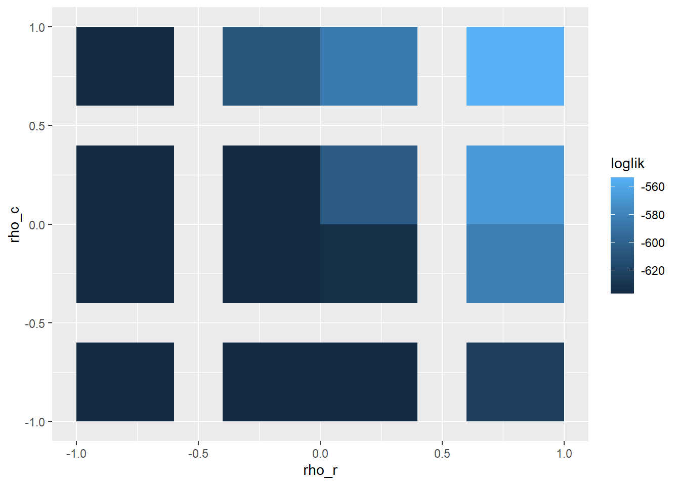

# Refine the grid around the most likely values (the range cannot contain exactly 1 or -1)
rho.grid <- expand.grid(rho_r = seq(0.5, 0.95, length = 4),
                        rho_c = seq(0.5, 0.95, length = 4))

5.6 Bayesian AR1xAR1

#library(INLA) 
## under construction....

5.7 Model Selection

Now that we have built these spatial models, how do we pick the right one? Unfortunately, there is no one model that works best in all circumstances. In addition, there is no single way for choosing the best model! Some approaches include:

1. comparing model fitness (e.g. AIC, BIC, log likelihood)
2. comparing post-hoc power (that is, the p-values for the treatments)
3. comparing standard error of the estimates

In order to make comparisons, the code below assembles all the model objects into one list. They are generated from different processes, as shown by the class attribute of each one, so this takes some data conditioning.

all.models <- mget(ls(pattern = "^nin_*"))
# print out their class
map(all.models, class)

## $nin.lme
## [1] "lme"
## 
## $nin_ar1ar1
## [1] "breedR"  "remlf90"
## 
## $nin_exp
## [1] "lme"
## 
## $nin_gaus
## [1] "lme"
## 
## $nin_lme
## [1] "lme"
## 
## $nin_matern
## [1] "lme"
## 
## $nin_sph
## [1] "lme"
## 
## $nin_spline
## [1] "SpATS"
## 
## $nin_trend
## [1] "lmerModLmerTest"
## attr(,"package")
## [1] "lmerTest"

5.7.1 Spatial dependence of residuals

It would be helpful to know if these methods were effective in reducing the spatial autocorrelation among the error residuals.

The function below extracts the residuals from each model and is needed because of different handling of missing values by the package SpATS.

L1 <- nrow(Nin)
non_na <- !is.na(Nin$yield)
L2 <- sum(non_na)

residuals <- map(all.models, function (x) {
  
  resids <- residuals(x)
  
  if(is.data.frame(resids)) {
    colnum = ncol(resids)
    resids = resids[,colnum]
  }
  
  if(length(resids) == L2) {
    resids_pl = rep(NA, L1)
    resids_pl[non_na] = resids
    resids = resids_pl
  }
  return(resids)
})

names(residuals) <- names(all.models)

Run a Moran’s I test on the extracted residuals:

library(spdep)

xy.rook <- cell2nb(nrow = max(Nin$row), ncol = max(Nin$col), type="rook")

Moran.I <- map_df(residuals, function(x) {
  mi = moran.test(x, nb2listw(xy.rook), na.action = na.exclude)
  mi.stat <- mi$estimate
  mi.stat$p.value <- mi$p.value
  return(mi.stat)
}) %>% mutate(model = names(all.models)) %>% dplyr::select(c(5, 1:4)) %>% 
  mutate_at(2:5, round, 4) %>% arrange(p.value)

Moran.I

## # A tibble: 9 × 5
##   model      `Moran I statistic` Expectation Variance p.value
##   <chr>                    <dbl>       <dbl>    <dbl>   <dbl>
## 1 nin.lme                 0.402      -0.0045   0.0025  0     
## 2 nin_exp                 0.756      -0.0045   0.0025  0     
## 3 nin_gaus                0.760      -0.0045   0.0025  0     
## 4 nin_lme                 0.402      -0.0045   0.0025  0     
## 5 nin_matern              0.760      -0.0045   0.0025  0     
## 6 nin_sph                 0.757      -0.0045   0.0025  0     
## 7 nin_trend               0.132      -0.0045   0.0025  0.0032
## 8 nin_spline             -0.0514     -0.0045   0.0025  0.826 
## 9 nin_ar1ar1             -0.112      -0.0045   0.0025  0.984

Only one model, nin_spline resulted in an improvement in Moran’s I. Nearest neighbor approaches can also improve Moran’s I. The significant p-values indicate that auto-correlation is still present in those models. However, that doesn’t mean the other models are ineffective. The other models incorporate the spatial auto-correlation directly into the error terms.

5.7.2 Compare Model Fit

log likelihood, AIC, BIC

Since these are not nested models, likelihood ratio tests cannot be performed. Log likelihood can be compared within the models from nlme but not across packages since they use different estimation procedures.

nlme_mods <- list(nin_lme, nin_trend, nin_exp, nin_gaus, nin_sph, nin_matern, nin_ar1ar1)

names(nlme_mods) <- c("LMM", "row-col_trend", "exponential", 
                        "gaussian", "spherical", "matern", "AR1xAR1")

data.frame(logLiklihood = sapply(nlme_mods, logLik),
           AIC = sapply(nlme_mods, AIC),
           BIC = sapply(nlme_mods, AIC, k = log(nrow(Nin_na)))) %>% arrange(desc(logLiklihood))

##               logLiklihood      AIC      BIC
## matern           -540.3386 1202.677 1410.788
## gaussian         -540.3401 1200.680 1405.379
## spherical        -541.7560 1203.512 1408.211
## exponential      -543.0149 1206.030 1410.729
## AR1xAR1          -550.4486 1104.897 1111.721
## row-col_trend    -577.6523 1275.305 1480.003
## LMM              -608.8508 1333.702 1531.577

Larger log likelihoods indicate a better fitting model to the data. A rule of thumb when comparing log likelihoods is that differences less than 2 are not considered notable. These results suggest that the Gaussian, spherical, power and Matérn models are substantially equivalent in capturing the variation present in this data set.

5.7.3 Experiment-wide error

exp_error <- as.data.frame(sapply(nlme_mods[-7], sigma))
exp_error

##               sapply(nlme_mods[-7], sigma)
## LMM                               7.041475
## row-col_trend                     4.754971
## exponential                       8.967355
## gaussian                          8.035251
## spherical                         7.946038
## matern                            8.061689

The overall experimental error, \(\sigma\), increased slightly in the correlated error models because field variation has been re-partitioned to the error when it was (erroneously) absorbed by the other experimental effects.

As a result, the coefficient of variation is not a good metric for evaluating the quality of spatial models.

CV = sapply(nlme_mods[-7], function(x) {
  sigma(x)/mean(fitted(x), na.rm = T) * 100
})
as.data.frame(CV)

##                     CV
## LMM           27.58441
## row-col_trend 18.62722
## exponential   35.99247
## gaussian      30.68459
## spherical     31.74386
## matern        30.81737

5.7.4 Post-hoc power

Simulation studies indicate that incorporating spatial correlation into field trial analysis can improve the overall power of the experiment (the probability of detecting true differences in treatments). When working with data from a completed experiment, power is a transformed p-value. Performing ANOVA can indicate which approach maximizes power.

anovas <- lapply(nlme_mods[-7], function(x){ 
  aov <- as.data.frame(anova(x))[2,]
  })

a <- bind_rows(anovas) %>% mutate(model = c("LMM", "row/column trend", "exponential", 
                                       "gaussian", "spherical", "matern")) %>% 
  arrange(desc(`p-value`)) %>% dplyr::select(c(model, 1:4)) %>% tibble::remove_rownames() 

a[6,2:5] <- anova(nin_trend)[3:6]
a

##              model numDF    denDF   F-value     p-value
## 1              LMM    55 165.0000 0.8754898 0.711852150
## 2         gaussian    55 165.0000 1.7815059 0.002816775
## 3           matern    55 165.0000 1.7816169 0.002814130
## 4      exponential    55 165.0000 1.8348864 0.001786539
## 5        spherical    55 165.0000 1.8370929 0.001752953
## 6 row/column trend    55 132.3739 1.3101069 0.107626854

This table indicates changes in the hypothesis test for “gen”. There is a dramatic change in power for this test when incorporating spatial covariance structures.

5.7.5 Standard error of treatment means

Retrieve predictions generated in the previous section:

#(standardise names for downstream merging step)
#preds_ar1ar1 <- preds_ar1ar1  %>% rename(emmean = "predicted.value", SE = "standard.error") 
all.preds <- mget(ls(pattern = "^preds_*")) 

Extract standard errors and plot:

errors <- lapply(all.preds, "[", "SE")
pred.names <- gsub("preds_", "", names(errors))
error_df <- bind_cols(errors)
colnames(error_df) <- pred.names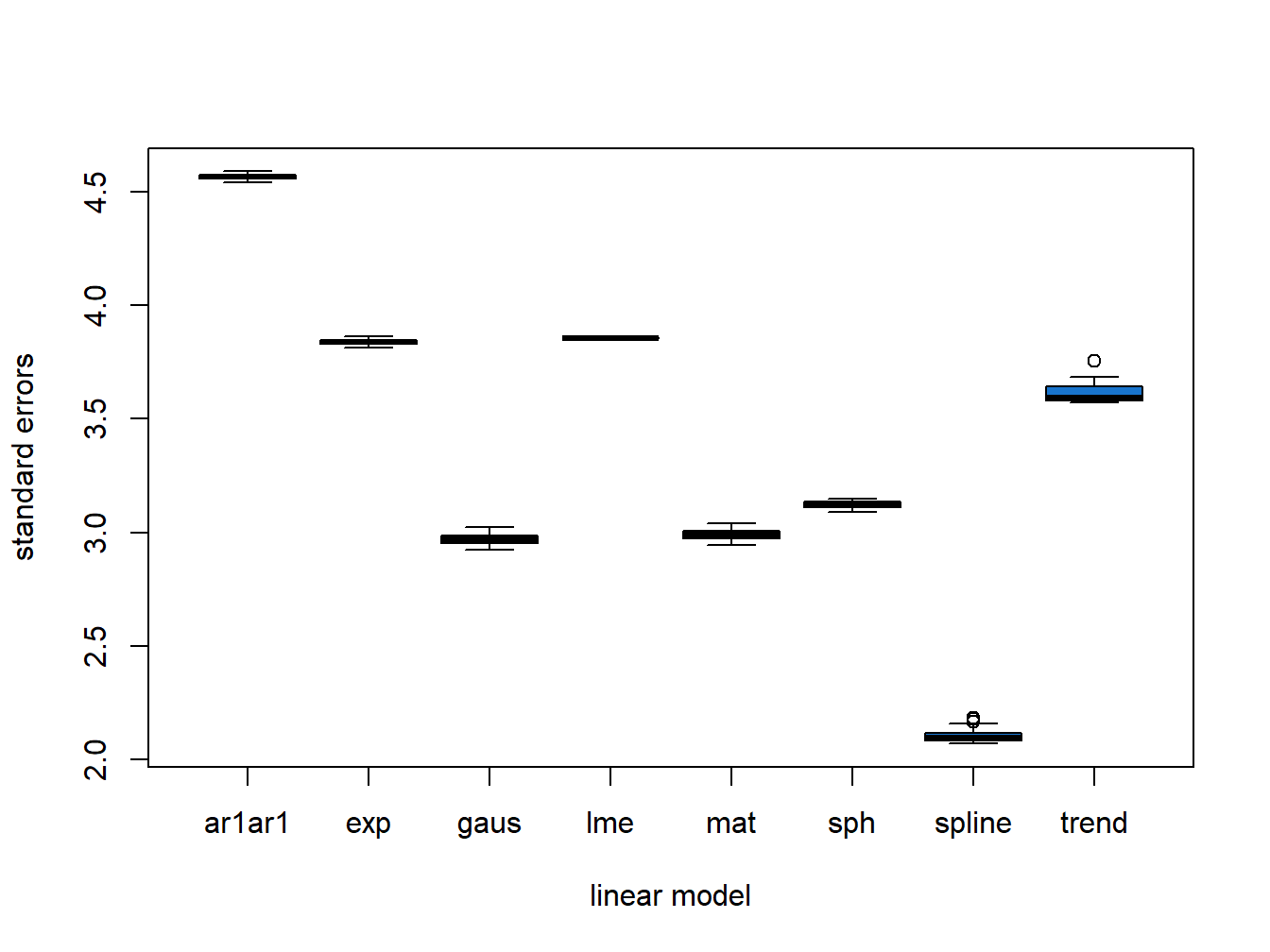

Figure 5.1: Differences in Variety Standard Error

5.7.6 Treatment means

Extract estimates:

preds <- lapply(all.preds, "[", "emmean")
preds_df <- bind_cols(preds)
colnames(preds_df) <- pred.names
preds_df$gen <- preds_exp$gen

Plot changes in ranks:

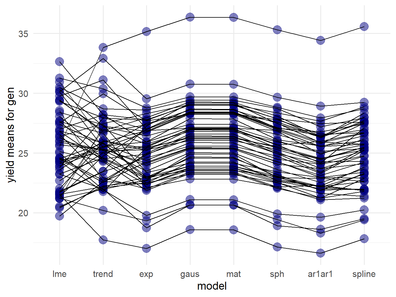
Figure 5.2: Differences in Variety Ranks

The black lines link the least squares means for a single variety. There is some consistency in the rankings between exponential, Gaussian, Matérn, and spherical covariance models. The control RCBD model, “lme”, has fundamentally different rankings. The spline and AR1xAR1 ranking are also sightly different from the other models.

Nevertheless, the following plot indicates considerable consensus in the least squares means from all of the spatial models. The upper diagonal contains Pearson correlations between those values.

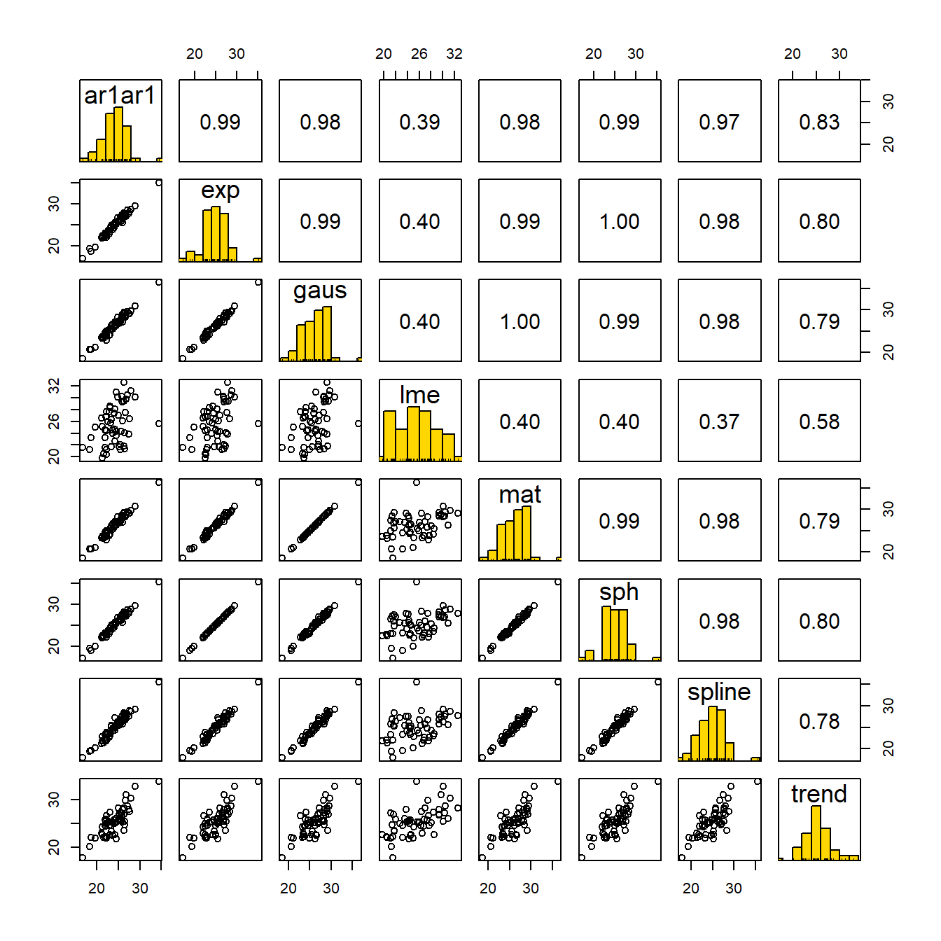
Figure 5.3: Correlations in Variety Means

5.8 Making decisions

There is no consensus on how to pick the best model. Some studies rely on log likelihood, while others seek to maximize the experimental power. Others have sought to minimize the root mean square error from cross validation.

The evidence suggest that for this data set, using any spatial model is better than running a naïve RCBD model.