Section 2 Introduction
2.1 Why care about spatial variation?
The goal of many agricultural field trials is to provide information about crop response to a set a treatments such as soil treatments, disease pressure or crop genetic variation. Agricultural field trials employ common experimental designs such as randomized complete block design to account for environmental heterogeneity. However, those techniques are quite often inadequate to fully account for spatial heterogeneity that arises due to field position, soil conditions, disease, wildlife impacts and more.

University Research Farm
When spatial autocorrelation is not accounted for in an analysis, the result can be incorrect treatment estimates, correlated errors (that violate the assumption of linear models and invalidate the analysis) and low experimental power. Incorporating spatial correlation between experimental plots can improve the overall accuracy and precision of these estimates.
2.2 Diagnosing spatial auto-correlation
Spatial correlation is similarity of plots that are close to one another. That correlation is expected to decline with distance. This is different from experiment-wide gradients, such as a salinity gradient or position on a slope.
2.2.1 Moran’s I
Moran’s I, sometimes called “Global Moran’s I” is similar to a correlation coefficient. It is a test for correlation between units (plots in our case).
\[ I = \frac{N}{W}\frac{\sum_i \sum_j w_{ij} (x_i - \bar{x})(x_j - \bar{x})}{\sum_i(x_i - \bar{x})^2} \qquad i \neq j\] and \(j\), x is the variable of interest, \(w_{ij}\) are a spatial weights between each \(i\) and \(j\), and W is the sum of all weights. The expected values of Moran’s I is \(-1/(N-1)\). Values greater than that indicate positive spatial correlation (areas close to each other are similar), while values less than the expected Moran’s I indicate dissimilarity as spatial distance between points decreases. Where N is total number of spatial locations indexed by \(i\)
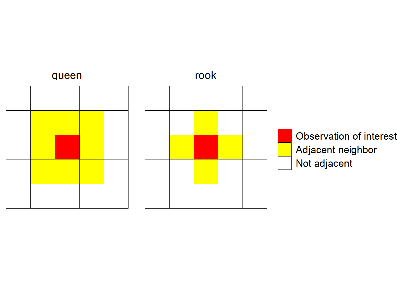
There are several options for defining adjacent neighbors and how to weight each neighbor’s influence. The two common configurations for defining neighbors are the rook and queen configurations. These are exactly what their chess analogy suggests: “rook” defines neighbors in an row/column fashion, while “queen” defines neighbors in a row/column configuration an also neighbors located diagonally at a 45 degree angle from the row/column neighbors. Determining this can be somewhat complicated when working with irregularly-placed data (e.g. county seats), but is quite unambiguous for lattice data common in planned field experiments:
Another test for diagnosing spatial correlation is Geary’s C:
\[ I = \frac{(N -1)}{2W}\frac{\sum_i \sum_j w_{ij} (x_i - x_j)^2}{\sum_i(x_i - \bar{x})^2} \qquad i \neq j\]
These terms have the same meaning in Moran’s I. The expected value of Geary’s C is 1. Values higher than 1 indicate positive spatial correlation and less than 1 indicate negative spatial correlation.
2.2.2 Empirical variogram & semivariance
An empirical variogram is a visual tool for understanding how error terms are related to each other over spatial distance. It relies on semivariance (\(\gamma\)), a statistic expressing variance as a function of pairwise distances between data points at points \(i\) and \(j\).
\[\gamma(h) = \frac{1}{2|N(h)|}\sum_{N(h)}(x_i - x_j)^2\]
Semivariances are binned for distance intervals. The average values for semivariance and distance interval can be fit to correlated error models such a exponential, spherical, Gaussian and Matérn. How to do this is explored further in 3 of this guide.
Three important concepts of an empirical variogram are nugget, sill and range
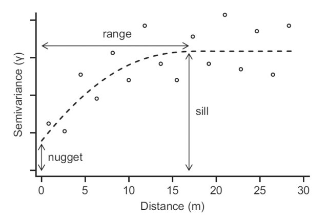
- range = distance up to which is there is spatial correlation
- sill = uncorrelated variance of the variable of interest
- nugget = measurement error, or short-distance spatial variance and other unaccounted for variance
2 other concepts:
- partial sill = sill - nugget
- nugget effect = the nugget/sill ratio, interpreted opposite of \(r^2\)