Section 3 Spatial Models
This section contains some of the statistical background behind why spatial models are used and how they work. Understanding this section is not essential, but it is extremely helpful. This section relies on information introduced in 2, so please make sure you have read that section if you are new to empirical variograms and spatial statistics.
General linear statistical models are commonly modeled as thus:
\[Y_i = \beta_0 + X_i\beta_1 + \epsilon_i\] \(\beta_1\) is a slope describing the relationship between a continuous variable and the dependent variable, \(Y_i\). If \(X_i\) is a categorical variable, such as a crop variety, then there will be \(p-1\) slopes estimated, where p is the number of unique treatments levels in \(X\).
The error terms, \(\epsilon_i\) are assumed normally distributed with a mean of zero and a variance of \(\sigma^2\) :
\[e_i ~\sim N(0, \sigma^2)\] The error terms, or residuals, are assumed to be identically and independently distributed (sometimes abbreviated “iid”). This implies a constant variance of the error terms and zero covariance between residuals.
If N = 3, the expanded model looks like this:
\[\left[ {\begin{array}{ccc} Y_1\\ Y_2\\ Y_3 \end{array} } \right] = \beta_0 + \left[ {\begin{array}{ccc} X_1\\ X_2\\ X_3 \end{array} } \right] \beta_1 + \left[ {\begin{array}{ccc} \epsilon_1\\ \epsilon_2\\ \epsilon_3 \end{array} } \right] \]
\[e_i ~\sim N \Bigg( 0, \left[ {\begin{array}{ccc} \sigma^2 & 0 & 0 \\ 0 & \sigma^2 & 0\\ 0 & 0 & \sigma^2\end{array} } \right] \Bigg) \]
If spatial variation is present, the off-diagonals of the variance-covariance matrix are not zero - hence the error terms are not independently distributed. As a result, hypotheses test and parameter estimates from uncorrected linear models will provide erroneous results.
3.1 Correlated error models
3.1.1 Distance-based correlation error models
There are mathematical tools for modelling how error terms are correlated with each other based on pairwise physical distance between observations. These models can be used to weight observations. Often, the data are assumed to be isotropic, where distance but not direction impacts the spatial error correlation.
There are several methods for estimating the semivariance as a direct function of distance.
3.1.1.1 Exponential
\[ \gamma (h)\left\{ {\begin{array}{cc} 0 & h = 0\\ C_0+C_1 \left [ 1-e^{-(\frac{h}{r})} \right] & h > 0 \end{array} } \right. \] where
\[ C_0 = nugget \\ C_1 = partial \: sill \\ r = range\]
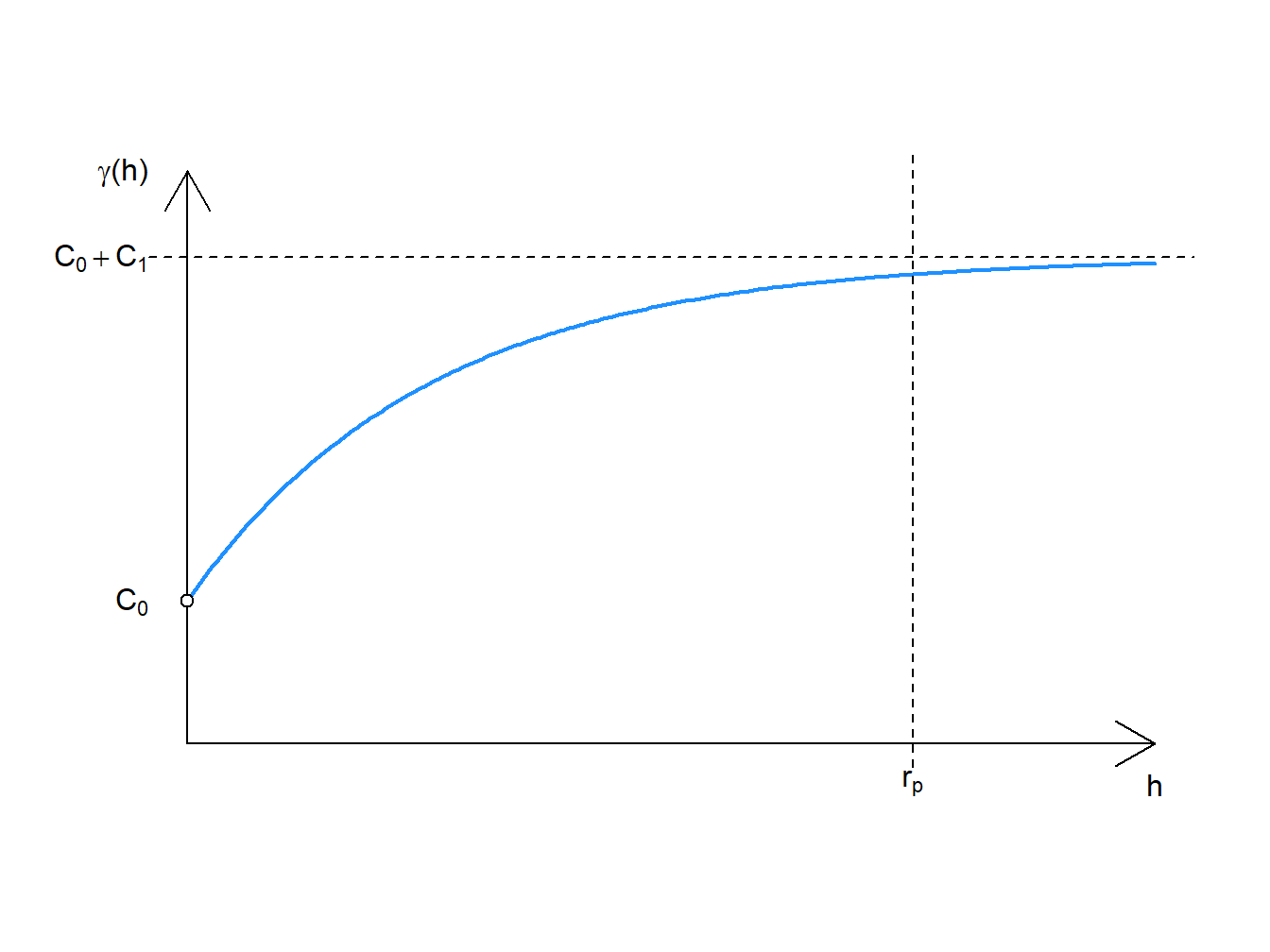
Figure 3.1: Exponential Model
\(3r = r_p\) is the “practical range”, which is 95% of the true value for \(C_1\).
3.1.1.2 Gaussian
(a squared version of the exponential model)
\[ \gamma (h)\left\{ {\begin{array}{cc} 0 & h = 0\\ C_0+C_1 \left [ 1-e^{-(\frac{h}{r})^2} \right] & h > 0 \end{array} } \right. \] where
\[ C_0 = nugget \\ C_1 = partial \: sill \\ r = range\]
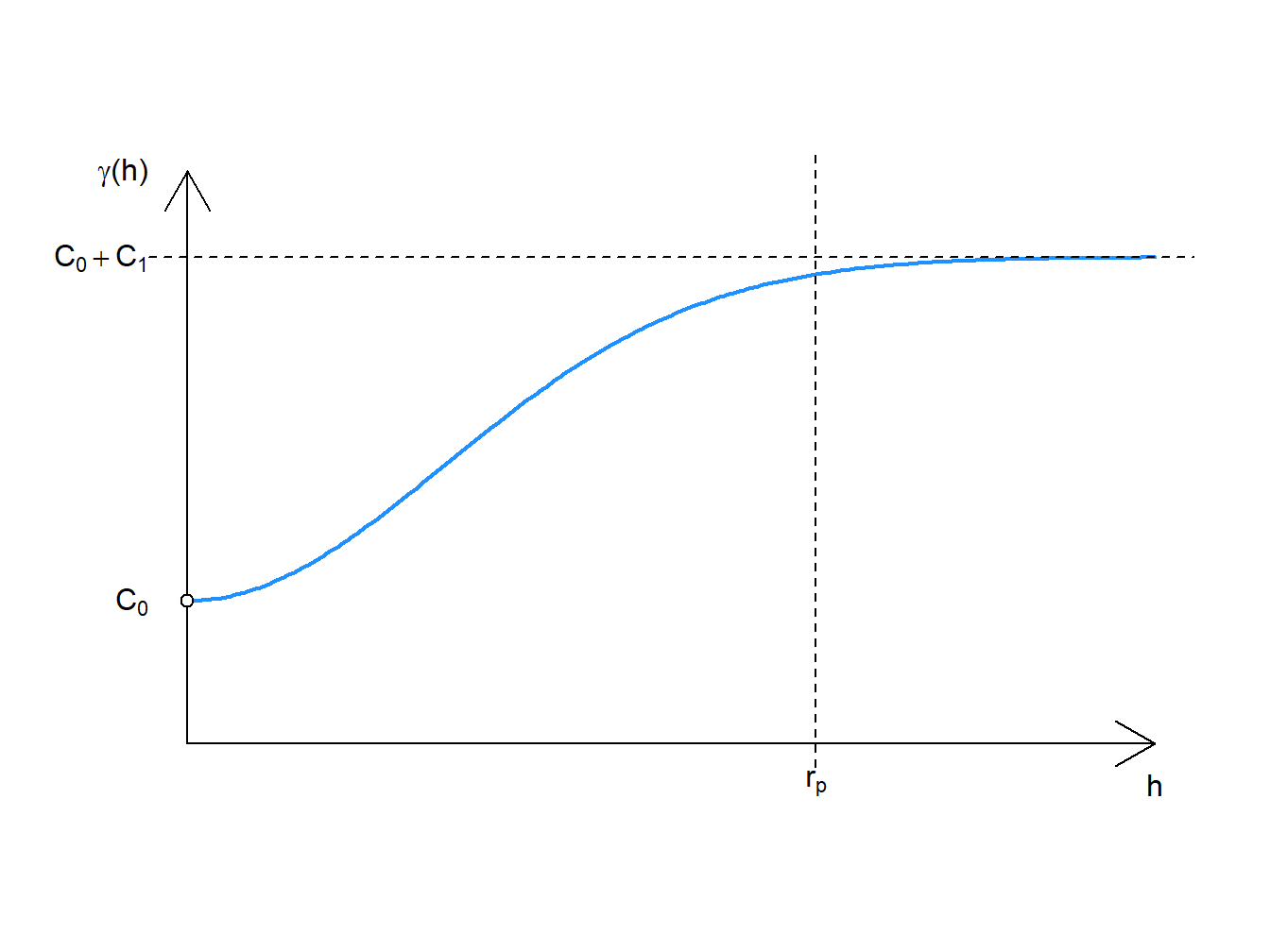
Figure 3.2: Gaussian Model
\(\sqrt 3r = r_p\) is the “practical range”, which is 95% of the true value for \(C_1\).
3.1.1.3 Spherical
\[ \gamma (h) = \left\{ {\begin{array}{cc} 0 & h = 0\\ C_0+C_1 \left[ \frac{3h}{2r}-0.5\bigg( \frac{h}{r}\bigg)^3 \right] & 0 <h \leq r \\ C_0 + C_1 & h > r \end{array} } \right. \] where
\[ C_0 = nugget \\ C_1 = partial \: sill \\ r = range\]
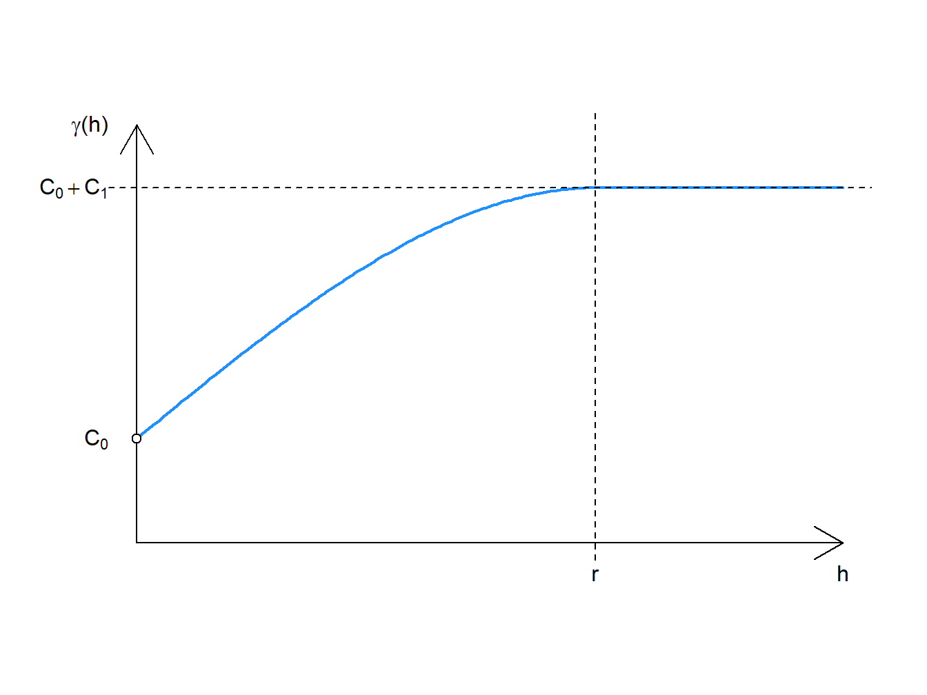
Figure 3.3: Spherical Model
3.1.1.5 Linear
\[ \gamma (h)=\left\{ {\begin{array}{cc} 0 & h = 0\\ C_0+C_1h & h > 0 \end{array} } \right. \] where
\[ C_0 = nugget \\ C_1 = slope \]
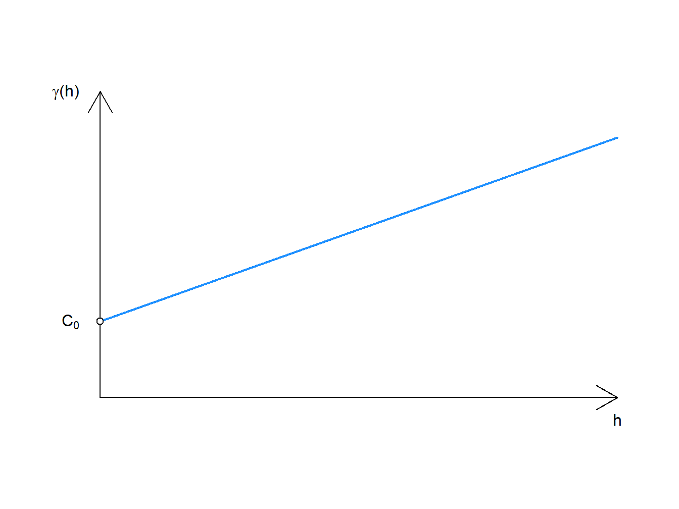
Figure 3.4: Linear Error Model
There is no sill or range in the linear model, so the variance will continue to increase as a function of distance.
3.1.1.6 Power
\[ \gamma (h)=\left\{ {\begin{array}{cc} 0 & h = 0\\ C_0+C_1h^\lambda & h > 0 \end{array} } \right. \] where
\[ 0 \leq \lambda <\leq 2 \\ C_0 = nugget \\ C_1 = scaling \: factor \]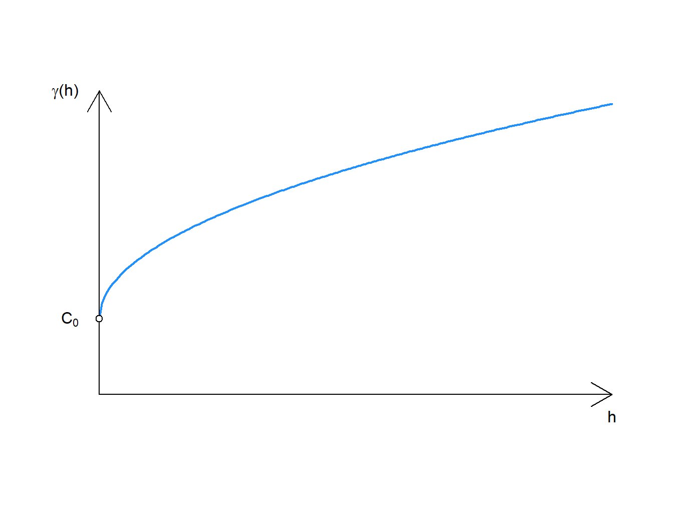
Figure 3.5: Power Model
When \(\lambda = 1\), that is equivalent to the linear model. Example above is when \(\lambda = 0.5\) (i.e. a square-root transformation) and \(C_1 = 1\). There is also no sill or range in the power model.
3.1.1.7 Matérn
\[\gamma(h) = c_0 + c_1 \bigg( 1- \frac{1}{2^{\kappa -1}\Gamma(\kappa)} \Big( \frac{h}{\alpha} \Big) ^{\kappa} K_\kappa \Big( \frac{h}{\alpha} \Big) \bigg)\]
Where
\[ C_0 = nugget \\ C_1 = partial \: scale \\ \alpha = smoothing \: factor \\ \kappa = covariance \: parameter \]
\(\Gamma(\kappa)\) is the gamma function:
\[\Gamma(\kappa) = (\kappa -1)!\]
and \(\kappa(\alpha)\) is a modified bessel function:
\[ K_\kappa(t) = \frac{\Gamma(\alpha)}{2} \big( \frac{t}{2} \big) ^{-\kappa}\]
3.1.2 Correlated error model for gridded data
Planned field experiments often have the advantage of being arranged in regular grid pattern that can be adequately described using Euclidean space. This simplifies aspects of understanding how error terms are related by distance since the data occur in evenly spaced increments. Furthermore, in many agricultural trials, there may be no interest in spatial interpolation between units. Some of the following models work with irregularly-spaced data, but the models below are simplified forms when the experimental units are arranged in regular grid.
For example, imagine an experiment consisting of 8 plots (plot = the experiment units) arranged in 2 rows, each with 4 ranges with this layout:
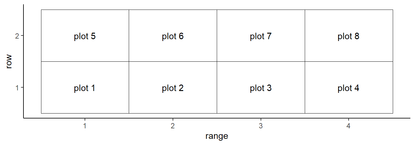
The statistical model for that experiment:
\[ \left[ {\begin{array} \ Y_1 \\ Y_2 \\ \vdots \\ Y_n \end{array} } \right] = \beta_0 + \left[ {\begin{array} \ X_1 \\ X_2 \\ \vdots \\ X_n \end{array} } \right] \beta_1 + \left[ {\begin{array} \ \epsilon_1 \\ \epsilon_2 \\ \vdots \\ \epsilon_n \end{array} } \right] \] \(X\beta\) refer to independent variable effects. This same model is also often presented in an abbreviated matrix form:
\[ \mathbf{Y = X\beta + \epsilon}\]
3.1.2.1 First order auto-regressive model (AR1)
This assumes that variance can be modelled as exponential function based on unit distance (e.g. row or range), either in a single direction or anistropic.
The AR1 structure across 2 rows is modeled as thus:
\[\mathbf { V_{AR(1)row}} = \sigma^2 \left[ {\begin{array}{cc} 1 & \rho \\ \rho & 1 \end{array} } \right] \otimes \mathbf{I_4}\]
This covariance model describes the correlation of observations in the row direction only.
And similarly the AR1 structure across 4 ranges is modeled as thus:
\[ \mathbf {V_{AR(1)range}} = \sigma^2 \left[ {\begin{array}{cccc} 1 & \rho & \rho^2 & \rho^3 \\ \rho & 1 & \rho & \rho^2 \\ \rho^2 & \rho & 1 & \rho \\ \rho^3 & \rho^2 & \rho & 1 \end{array} } \right] \otimes \mathbf{I_2} \]
This covariance model describes the correlation of observations in the range direction only.
In combined AR1xAR1 model, the parameter, \(\rho\) may need to estimated separated across the row and column directions depending on the shape of the plots and site-specific field variation. Very rectangular plots are likely to require a separate estimate of the \(\rho\) parameter for each direction.
\[\begin{equation} \mathbf {V_{AR(1)row} \otimes V_{AR(1)range}} = \sigma^2 \left[ {\begin{array}{cccc | cccc} 1 & \rho_1 & \rho_1^2 & \rho_1^3 & \rho_2 & \rho_1\rho_2 & \rho_1^2\rho_2 & \rho_1^3\rho_2 \\ \rho_1 & 1 & \rho_1 & \rho_1^2 & \rho_1\rho_2 & \rho_2 & \rho_1\rho_2 & \rho_1^2\rho_2\\ \rho_1^2 & \rho_1 & 1 & \rho_1 & \rho_1^2\rho_2 & \rho_1\rho_2 & \rho_2 & \rho_1\rho_2\\ \rho_1^3 & \rho_1^2 & \rho_1 & 1 & \rho_1^3\rho_2 & \rho_1^2\rho_2 & \rho_1\rho_2 & \rho_2 \\ \hline \rho_2 & \rho_1\rho_2 & \rho_1^2\rho_2 & \rho_1^3\rho_2 & 1 & \rho_1 & \rho_1^2 & \rho_1^3 \\ \rho_1\rho_2 & \rho_2 & \rho_1\rho_2 & \rho_1^2\rho_2 & \rho_1 & 1 & \rho_1 & \rho_1^2 \\ \rho_1^2\rho_2 & \rho_1\rho_2 & \rho_2 & \rho_1\rho_2 & \rho_1^2 & \rho_1 & 1 & \rho_1 \\ \rho_1^3\rho_2 & \rho_1^2\rho_2 & \rho_1\rho_2 & \rho_2 &\rho_1^3 & \rho_1^2 & \rho_1 & 1 \\ \end{array} } \right] \end{equation}\]
Note: \(\rho_1\) and \(\rho_2\) are the parameter estimate for \(V_{AR1(1) row}\) and \(V_{AR(1)range}\), respectively.
Please note that these error models are for modelling localised variation based on physical proximity. It is assumed that eventually a distance in the experiment can be reached in which 2 observations can be treated independent.
If there are spatial trends that extend along the entire scope of an experiment (for instance, due to position on a slope), then an additional trend analysis should be conducted.
3.2 Spatial Regression methods
These approaches look use information from adjacent plots to adjust for spatial auto-correlation.
3.2.1 Spatial autoregressive (SAR)
Sometimes called a “lag” model, the SAR model uses correlations with neighboring plots dependent variable to predict Y. The auto-regressive model explicitly models correlations between neighboring points.
\[\mathbf{Y = \rho W Y + X\beta + \epsilon} \]
While this may look strange, \(\mathbf{W}\) is an \(n\) x \(n\) matrix weighting the neighbors with a diagonal of zero so the value at \(i=j\), that is \(Y_{ijk}\) itself, is not used on the right-hand side to predict \(Y_{ijk}\) on the left-hand side of the equation. The error terms are assumed iid.
On Weights
Setting weights of neighbors is dealt with in the next chapter 5.
3.3 Trend analysis
3.3.1 Row and column trends
Experiment wide-trends should be modeled with directional trend models. These are comparatively simple models:
\[Y_{ijk} = \beta_0 + X_{i1}\beta_1 + Row_{j2}\beta_2 + Range_{k3}\beta_3 +\epsilon_{ijk}\]
If the assumption of independent, normal, and identical errors are met, then this model will suffice. If spatial variation is still present, additional measures will need to be taken.