library(dplyr); library(tidyr)Introduction to Data Wrangling
Learning Goals
At the end of this lesson, you should:
- be able to select columns in R using
select() - be able to filter a data set using
filter() - be aware of how to conditionally create new variables using
case_when() - know to create new variables using
mutate() - be able to rename variables using
rename() - be able to sort a data set using
arrange() - understand how to handle missing values with
drop_na(),na_if()andreplace_na() - be able to use
separate()to split up single variables into multiple variables
First, load libraries:
Next, import data:
variety_trials <- read.csv(here::here("data", "trial_data.csv"))
weather <- read.csv(here::here("data", "weather_data.csv"))
What is going on with
here::here()?
The here() function is from the here package. This package simplifies working directory issues by setting it to where the nearest .Rproj files exists. When using a .qmd file, it looks for the .Rproj file that is the same directory as that file and moves up the directory tree.
Tidyverse notes
This lesson relies on group of packages called the “Tidyverse”, in particular dplyr and tidyr.
These packages follow a special set of rules called “non-standard evaluation” (sometimes abbreviated “NSE”). Tidyverse non-standard evaluation uses quotes far less often than “base R” (base R are package that are installed automatically when R is updated). It also uses indexing $ less frequently. You can name a variable directly instead of using dataset$var.
Many functions in the Tidyverse follow this structure:
function(dataset, action)
Where “dataset” is the data framed being input and “action” is whatever action is being taken.
Selecting columns
The function select is used to specify column you want to keep (all rows are returned). Columns can be specified by name or position (i.e. the first two columns in the data set would be 1:2).
Select by name:
select1 <- select(variety_trials, variety, yield, grain_protein)
head(select1)
variety yield grain_protein
1 12SB0197 71.69333 9.8325
2 12SB0197 108.60301 9.6025
3 12SB0197 81.71237 11.2700
4 12SB0197 103.84303 10.3500
5 Jefferson 65.26589 10.2350
6 Jefferson 104.37355 11.0400You can also select on what columns you do not want:
select2 <- select(variety_trials, -trial)
select3 <- select(variety_trials, -c(trial))

head(select2); head(select3)
rep variety yield grain_protein test_weight
1 1 12SB0197 71.69333 9.8325 62.1
2 2 12SB0197 108.60301 9.6025 64.2
3 3 12SB0197 81.71237 11.2700 65.6
4 4 12SB0197 103.84303 10.3500 64.3
5 1 Jefferson 65.26589 10.2350 62.8
6 2 Jefferson 104.37355 11.0400 65.2 rep variety yield grain_protein test_weight
1 1 12SB0197 71.69333 9.8325 62.1
2 2 12SB0197 108.60301 9.6025 64.2
3 3 12SB0197 81.71237 11.2700 65.6
4 4 12SB0197 103.84303 10.3500 64.3
5 1 Jefferson 65.26589 10.2350 62.8
6 2 Jefferson 104.37355 11.0400 65.2
Note
The variables specified in select() will appear in the new data frame in exactly the order they were listed in the function call.
Sometimes, you might want to select many columns that share something common about their name:
select4 <- select(variety_trials, starts_with("r"))
head(select4)
rep
1 1
2 2
3 3
4 4
5 1
6 2This particular example is not all that useful, but you might have a large data set, with several dozen variables that all start with “snp” followed by some alpha-numeric code (e.g. “snp4738”). This function will enable you to select these column more efficiently than naming every single one.
There are more options for pattern matching on column names:
?tidyselect::starts_with #another option for searching help from the R console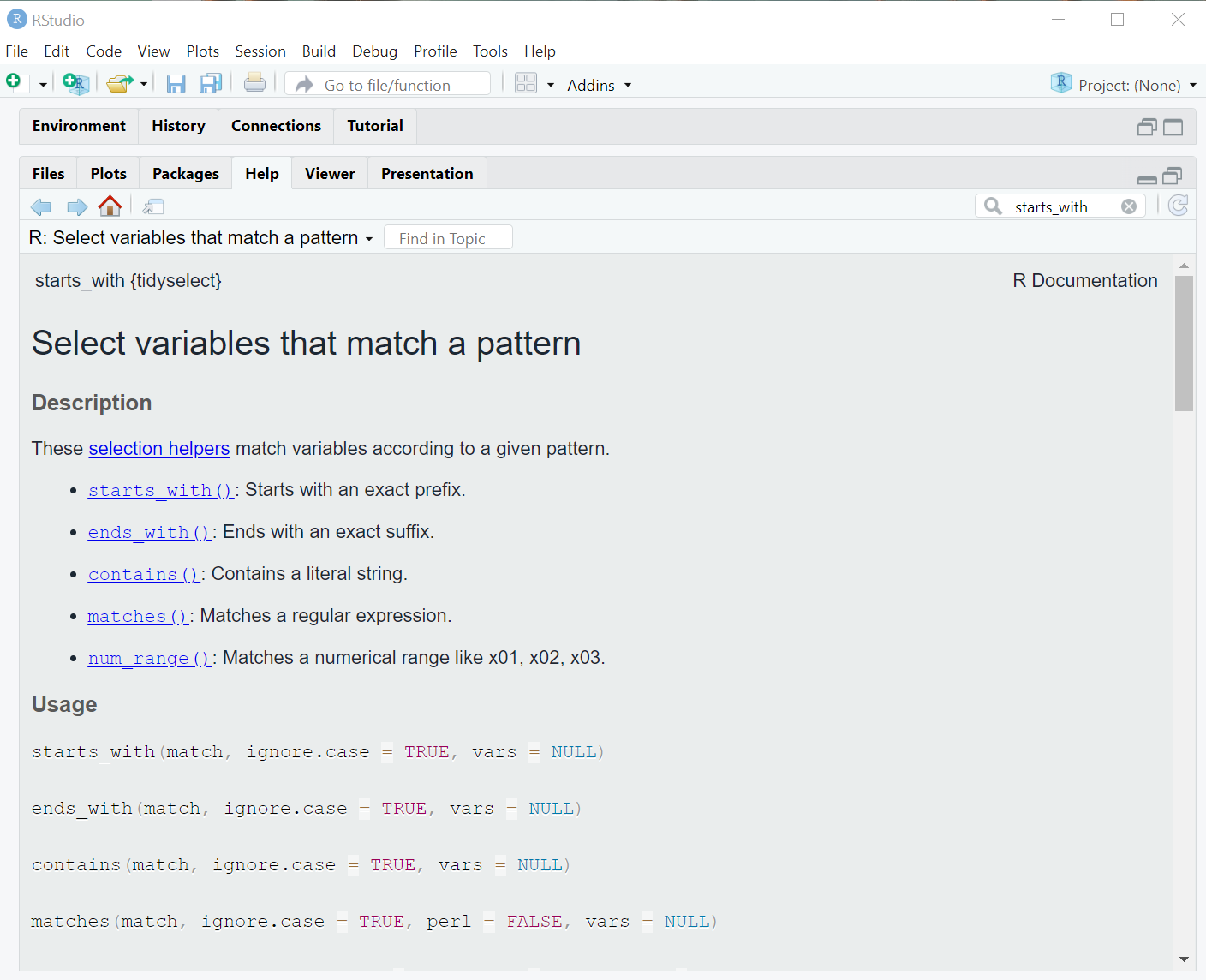
Filtering rows
The function filter is used to specify rows you want to keep (all columns are returned). This command uses logical operators for deciding what to keep.
filter1 <- filter(variety_trials, variety == "Stephens") # match one name
filter2 <- filter(variety_trials, variety %in% c("Stephens", "Bobtail")) # match multiple names
filter3 <- filter(variety_trials, yield > 50 & grain_protein <= 14) # filter on multiple conditions

dim(filter1); dim(filter2); dim(filter3)
[1] 4 6[1] 16 6[1] 1017 6
Note
It is also possible to select by numeric position:
select(variety_trials, c(1:3, 4))While selecting by numeric position works, it is an unreliable choice because it depends on column order or row order being exactly as you expect it. This may work the first time you write + run code, but it is likely to fail over time as you sort, augment or change data sets.
Practice Problems
Import “trial_data.csv” with the readr function
read_csv().Select columns that contain “i” in the column name and assign it a name “select_colm”.
Using the object from importing “trial_data.csv”, filter when variety is “Jefferson” and “Dayn”, and yield greater than or equal to 70. Assign these results to a new object.
Creating new variables
You can quite create new variables with a mutate() function call:
mutate(dataset, var_name = variable)
Examples:
## Create a new column
mutate1 <- mutate(variety_trials,
                    dataset = "example")

mutate1 <- mutate(mutate1,
                     row_position = 1:n())

## use existing column with different name
mutate1 <- mutate(mutate1,
                    trial_id = trial)

## calculate a new variable
mutate1 <- mutate(mutate1,
                    yield_new = yield+50)

mutate1 <- mutate(mutate1,
                    yield_protein = yield + grain_protein)

## change class of existing variable
mutate1 <- mutate(mutate1,
                    rep_factor = as.factor(rep))

head(mutate1)
trial rep variety yield grain_protein test_weight
1 SWIdahoCereals_H_S_PAR_2018 1 12SB0197 71.69333 9.8325 62.1
2 SWIdahoCereals_H_S_PAR_2018 2 12SB0197 108.60301 9.6025 64.2
3 SWIdahoCereals_H_S_PAR_2018 3 12SB0197 81.71237 11.2700 65.6
4 SWIdahoCereals_H_S_PAR_2018 4 12SB0197 103.84303 10.3500 64.3
5 SWIdahoCereals_H_S_PAR_2018 1 Jefferson 65.26589 10.2350 62.8
6 SWIdahoCereals_H_S_PAR_2018 2 Jefferson 104.37355 11.0400 65.2
dataset row_position trial_id yield_new yield_protein
1 example 1 SWIdahoCereals_H_S_PAR_2018 121.6933 81.52583
2 example 2 SWIdahoCereals_H_S_PAR_2018 158.6030 118.20551
3 example 3 SWIdahoCereals_H_S_PAR_2018 131.7124 92.98237
4 example 4 SWIdahoCereals_H_S_PAR_2018 153.8430 114.19303
5 example 5 SWIdahoCereals_H_S_PAR_2018 115.2659 75.50089
6 example 6 SWIdahoCereals_H_S_PAR_2018 154.3736 115.41355
rep_factor
1 1
2 2
3 3
4 4
5 1
6 2All the above performed tasks can we done in one go.
mutate2 <- mutate(variety_trials,
                    dataset = "example",
                    row_position = 1:n(),
                    trial_id = trial,
                    yield_new = yield+50,
                    yield_protein = yield + grain_protein,
                   rep_factor = as.factor(rep))
This created 6 new variables:
- dataset which is a character with the value “example” for all rows
- row_position providing the row number, starting at 1 and ending at
n(), a function that returns the total nubmer of rows in the data frame - trial_id, renamed the trial column.
- yield_new which is the sum of the value for yield plus 50.
- yield_protein the addition of two variables in the data set (this is also vectorized, calculating this for each row)
- rep_factor which is a new column to represent the replicate, but the class of a new variable is ‘factor’ instead of ‘numeric’.
These example cover the majority of what you are likely to experience: creating a constant, calculating new variables from existing variables, pulling in an external variables, and so forth.
This is equivalent to what was taught earlier using $ notation:
mutate1 <- variety_trials # first, copy the data frame
mutate1$dateset <- "example"
mutate1$row_position <- 1:nrow(mutate1)
mutate1$trial_new <- mutate1$trial # note that NSE cannot be used
mutate1$random_yield <- mutate1$yield + rnorm(nrow(mutate1))
mutate1$binom_var = new_var
mutate1$yield_protein <- mutate1$yield + mutate1$grain_protein
This can be a bit longer and cumbersome compared to mutate statements, but it does work.
case_when(), a special addition to mutate statements
Occasionally, you will need a define a variable conditionally, based on information from other variables. Here is an example for variety trial data. Here, a special minimum value is created where all data for “yield” less than 100 are set at 100:
Var1 <- mutate(variety_trials, new_min = case_when(
  yield <= 100 ~ 100,
  TRUE ~ yield))
head(Var1)
Everything to the left of the tilde ~ is a logical expression to evaluate. Everything to the right of the tilde is the value to put if the logical expression evaluates to TRUE.
This can easily become more complex with the addition of other logical expressions and categorical levels to create.
If you have a categorical variable that needs further refinement (e.g. collapsing of multiple levels into one), check out the package forcats, which provides many functions for manipulating categorical (factor or character) variables.
Renaming Variables
Compared to mutate(), the function for renaming variables, rename(), is a breeze!
rename(dataset, new_name = "old_name")This is similar to variable assignment:
new_name <- old_nameExcept that quotes are always used when specifying the old variable name.
Example:
rename1 <- rename(variety_trials, cultivar = "variety")
head(rename1, 3)
trial rep cultivar yield grain_protein test_weight
1 SWIdahoCereals_H_S_PAR_2018 1 12SB0197 71.69333 9.8325 62.1
2 SWIdahoCereals_H_S_PAR_2018 2 12SB0197 108.60301 9.6025 64.2
3 SWIdahoCereals_H_S_PAR_2018 3 12SB0197 81.71237 11.2700 65.6Also, you can use rename notation in select statements:
rename2 <- select(variety_trials, cultivar = "variety", yield, protein = "grain_protein")This function selected the columns “variety”, “yield” and “grain_protein”, while renaming “variety to”cultivar” and “grain_protein” to “protein” - a handy shortcut.
Split up variables
You may encounter variables with information about multiple things. In agriculture, I see variables with values such as “Moscow_2021”, “Moscow_2022”, “StJohn_2021”, “StJohn_2022”. This variables is indicating multiple things - location and year in this exmample. This is a useful variable by itself, but a researcher might want to separate out location and year for other analytical purposes. The tidyr function separate() can do that.
The first column of “variety_trials” contains considerable information, all separated by an underscore:
variety_trials$trial[1][1] "SWIdahoCereals_H_S_PAR_2018"The first term is the program conducting the trial, the second is the crop grown, the third term is a location code, and the last term is the year. Let’s separate those terms into separate columns/variables.
Before running a separate() command, always check the variable to make sure it is structured as you expect.
Use distinct() to determine the unique observations for the column “trial” in the the object “variety_trials”.
distinct(variety_trials, trial) trial
1 SWIdahoCereals_H_S_PAR_2018
2 SWIdahoCereals_H_S_WEI_2018
3 SWIdahoCereals_H_W_PAR_2017
4 SWIdahoCereals_H_W_PAR_2018
5 SWIdahoCereals_H_W_WEI_2018
6 SWIdahoCereals_HRS_PAR_2016
7 SWIdahoCereals_HRS_PAR_2017
8 SWIdahoCereals_HRS_PAR_2019
9 SWIdahoCereals_HRS_PAR_2020
10 SWIdahoCereals_HRW_PAR_2019
11 SWIdahoCereals_HRW_PAR_2020
12 SWIdahoCereals_HWS_PAR_2016
13 SWIdahoCereals_HWS_PAR_2017
14 SWIdahoCereals_HWS_PAR_2019
15 SWIdahoCereals_HWS_PAR_2020
16 SWIdahoCereals_HWW_PAR_2019
17 SWIdahoCereals_HWW_PAR_2020
18 SWIdahoCereals_SWS_PAR_2016
19 SWIdahoCereals_SWS_PAR_2017
20 SWIdahoCereals_SWS_PAR_2018
21 SWIdahoCereals_SWS_PAR_2019
22 SWIdahoCereals_SWS_PAR_2020
23 SWIdahoCereals_SWS_WEI_2018
24 SWIdahoCereals_SWW_PAR_2017
25 SWIdahoCereals_SWW_PAR_2018
26 SWIdahoCereals_SWW_PAR_2019
27 SWIdahoCereals_SWW_PAR_2020
28 SWIdahoCereals_SWW_WEI_2018The variable variety_trials$trial uses an underscore to separate its components. However, one of the terms we mean to keep as one component does have an underscore inside of it, which will interpreted incorrectly as a term separator. The function gsub() can be used to fix this.
variety_trials$trial <- gsub(pattern = "_H_", replacement = "_H-", x = variety_trials$trial)Now, separate() will split the variable into 4 components:
variety_trials <- separate(variety_trials, trial,
                           into = c("program", "crop", "location", "year"),
                           sep = "_",
                           remove = FALSE)
The argument remove = FALSE indicates that we want to keep the input variable (“trial”). By default, it would be removed.
The opposite function is tidyr::unite() which will paste these variable together, separate by any character string you specify. unite() also can ignore missing data when pasting information together, avoiding this unfortunate result: “some.var_NA_NA_another.var”. You would get “some.var_another.var” instead.
Practice Problems
- Import “weather.csv” with the
readr::read_csv(). - Create a new variable named T_avg as an average of ‘tmin_F’ and ‘tmax_F’ using a
mutate()function and name this data frame as ‘weather1’. - Select “name” column from the weather1 data set and rename it as “location”.
- In weather1 data set, select the first five columns and reduce that data set to unique rows (look into using
distinct()for extracting the unique observations). - Using weather1 data set, create a new variable as combination of station and name variables separated by “_” (e.g. station_name) using the unite() function.
Tip: search for unite() in help.
Functions for Missing Data
Remove missing data
dplyr::filter() can be used to filter missing data, but tidyr has a function, drop_na() that makes this easier. You can filter out rows based on missing data in any number of columns, including all columns. Note that this works on observations R has designated as NA. If an observation has white space instead of NA after data import into R, those are not equivalent.
This will remove all rows with any missing data.
na_filter_ex1 <- drop_na(variety_trials)This will remove rows with missing data in ‘grain_protein’ and ‘test_weight’.
na_filter_ex2 <- drop_na(variety_trials, grain_protein, test_weight)Designate missing data
Sometimes, you may have some odd observations you would like designated as missing. This can be accomplished with the mutate() function, but sometimes this shortcut is preferred. na_if() works on vectors, within a data frame or by itself.
trial_data <- mutate(variety_trials, var2 = na_if(variety, "Dayn"))
# check that it worked as intended:
filter(trial_data, var2 == "Dayn")
[1] trial program crop location year
[6] rep variety yield grain_protein test_weight
[11] var2
<0 rows> (or 0-length row.names)This also might be useful if specific columns use ‘-9’ to indicate missing values:
# not that this demonstration code will not change the data frame because we did not use -
variety_trial <- mutate(variety_trials, yield2 = na_if(trial, "-9"))
Replace missing data with a value
There are other moments that you may want to replace missing values with something in particular (perhaps zero, but be cautious when doing so). replace_na() can accomplish this. Like na_if(), this function operates on vectors.
variety_trials <- mutate(variety_trials, protein = replace_na(grain_protein, -9))
# check that it worked as intended:
hist(variety_trials$protein)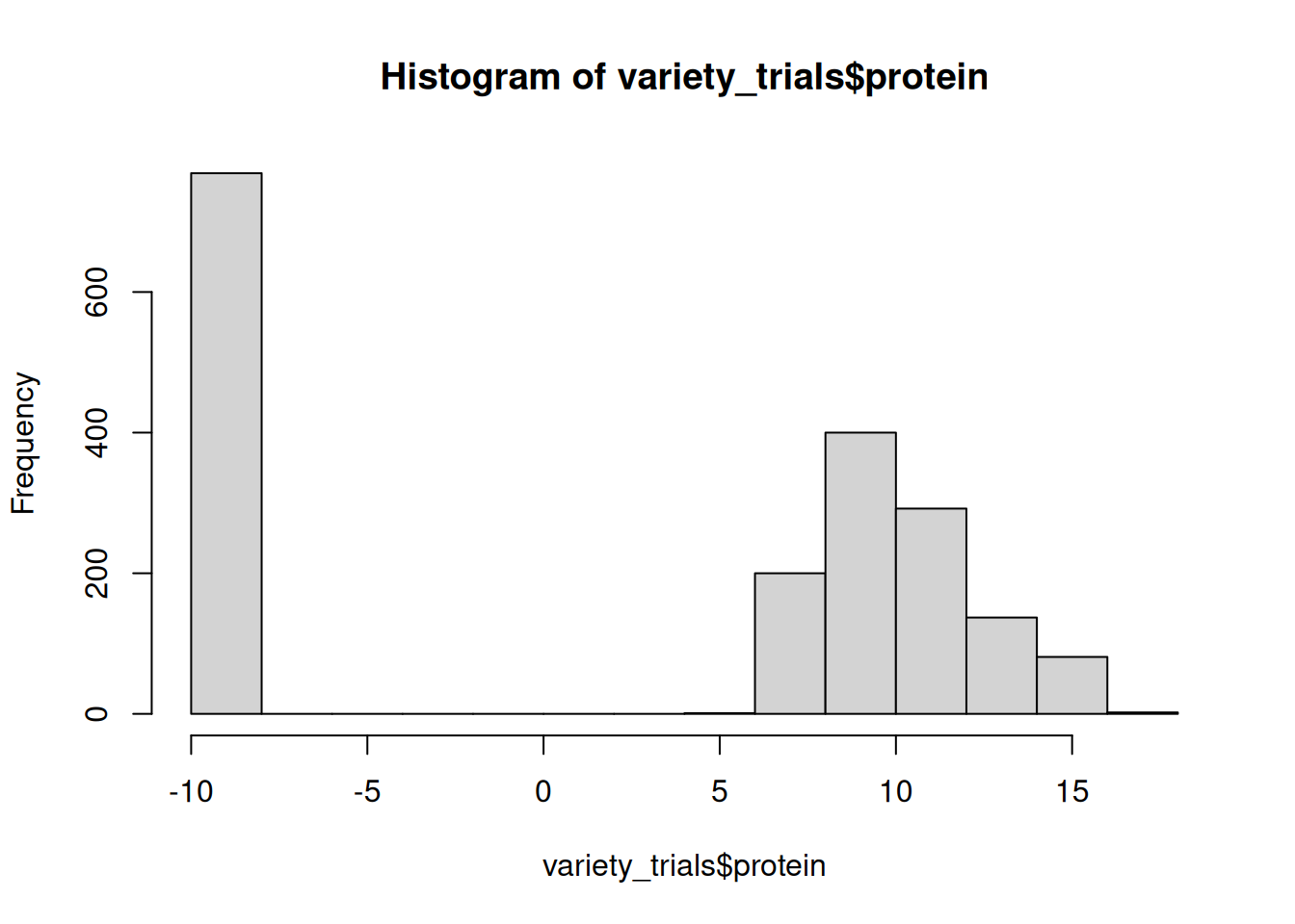
Sometimes, data sets have clear indications when a values is intended to be filled:
data1 <- data.frame(experiment = c("exp1", NA, NA, NA, "exp2", NA, NA, NA),
                    observation = rnorm(n = 8, mean = 50, sd = 1))
data1
experiment observation
1 exp1 49.95564
2 <NA> 50.86628
3 <NA> 49.80932
4 <NA> 50.63598
5 exp2 51.40040
6 <NA> 51.41618
7 <NA> 50.10544
8 <NA> 48.88690data2 <- fill(data1, experiment, .direction = "down")
data2 experiment observation
1 exp1 49.95564
2 exp1 50.86628
3 exp1 49.80932
4 exp1 50.63598
5 exp2 51.40040
6 exp2 51.41618
7 exp2 50.10544
8 exp2 48.88690Sorting a data set
Prior to dplyr, sorting in R was a nightmare. Excel makes this so easy! Why was R torturing us??? But, dplyr has made this much easier:
arrange(dataset, variable1, variable2, ....)You can sort on as many variables as you like! It will sort on the first variables listed and within that, the second variable listed, and so on.
Example;
arrange1 <- arrange(variety_trials, variety, yield)Output file
Let’s output this object to file so we can use it later.
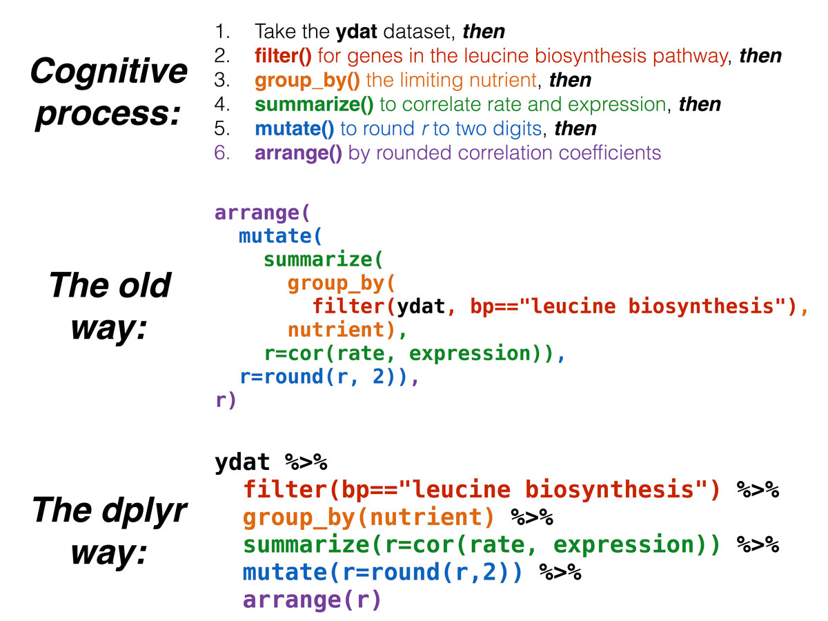
write.csv(variety_trials, here::here("outputs", "variety_trials_clean.csv"), row.names = FALSE)The pipe
The pipe operator %>% or its newer replacement |> are magic, or at least, they make our (data wrangling) lives so much easier.
The pipe operator works as thus:
operation_1 %>% operation_2One operation can be performed (e.g. a select() command), and that resulting data frame is passed on to the next operation (e.g. filter()).
Example: filter then sort
pipe1 <- filter(variety_trials, yield < 75) %>% arrange(variety)The data set is not named in the second operation because it is assumed to be dataset provided in the first operation. Whatever is being output directly left of the pipe operator is in the input data set.
We can take this even further by making the first operation our addition of the data set to the pipes:
pipe2 <- variety_trials %>% filter(yield < 75) %>% arrange(variety)The pipe has made data wrangling so much easier! Before the pipe, each of these operations can be specified separately with its own object. So when you were done, you had roughly 50 objects in your environment, 48 of which were not needed anymore.
It also saved us from the “parentheses cascade” where one function is nested inside another function, which is nested within another, and so forth. It can be difficult to ascertain what parentheses belong to what operation, which often leads to coding errors. In a set of nestd functions, the inner functions are first executed and the outer functions are executed last. no longer had any sense of which set of parentheses belong to which operation.
Practice Problems
Using piping, import “trial_metadata.csv”, filter by 2 nurseries of your choosing, then sort by year and planting date
Putting it all together
What going on this notation?
tibble::rownames_to_column()This is a normal function call (the function being rownames_to_column()), and it is specifying that the package where this function resides is tibble (a tibble is the Tidyverse alternative to the data frame).
You want to use this notation in 2 circumstance:
You don’t want to load the entire package with a
library()call, especially if you only need one function from itThe name of the function you want to call from a package conflicts with function names from another package. A very common example is
filter()- this is a dplyr function, but it is also a base R function. Sometimes, you may receive a very puzzling error when usingfilter()that essentially is indicating that the wrong package was used. Using notation likedplyr::filter()clarified to R that you want to use the dplyr version offilter(). By default, the most recent package loaded overrides other function name conflicts, but sometiimes, it’s helpful to be unambiguous in your R function calls.