library(readr); library(dplyr); library(tidyr)

metadata <-  read_csv(here::here("data", "trial_metadata.csv"), show_col_types = FALSE)

variety_trial <- read.csv(here::here("data", "trial_data.csv"))

genotypes <- read_csv(here::here("data", "genotypic_data_rotated.csv"), show_col_types = FALSE)Combining Data Sets
Learning Goals
At the end of this lesson, you should:
- understand the concept of a “key” for merging
- be able to merge two data sets together
- know the difference between left join, right join, full join, semi-join and anti-join
As usual, let’s start by importing data
Before working on merging and binding data sets, let’s create two subsets from the “variety_trial” data set. Here, we are using the filter() and select() functions to create two smaller data sets. We have created two data sets, where each contain a single trial and selected matching columns.
trial_1 <- variety_trial %>% filter(trial == "SWIdahoCereals_HRS_PAR_2016") %>% select(trial, rep, variety, yield)

trial_2 <- variety_trial %>% filter(trial == "SWIdahoCereals_SWS_PAR_2018") %>% select(trial, variety, rep, grain_protein)
For merging, it is done in groups of two; that is, two tables at a time are merged together.
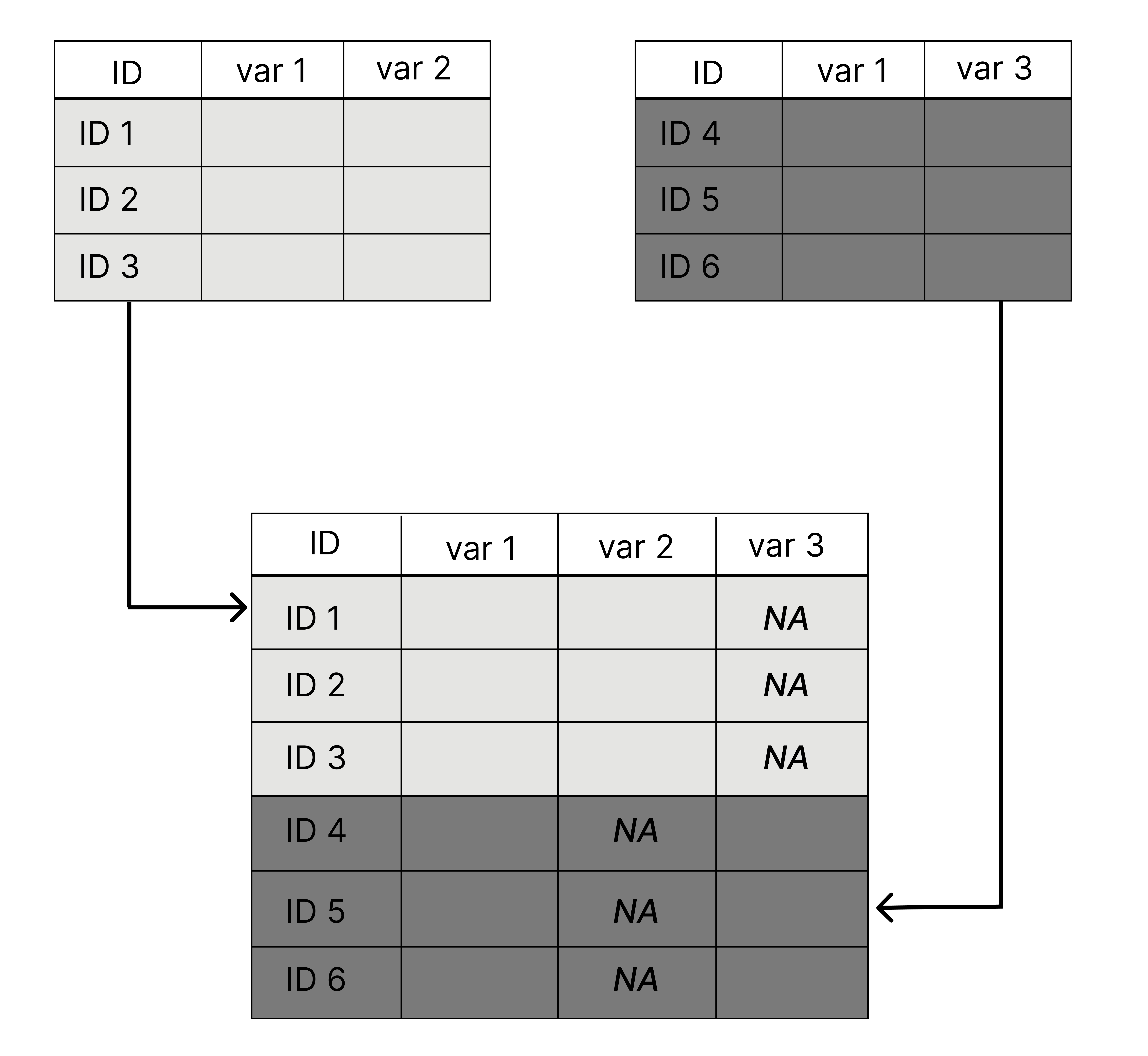
Bind rows
If you have two data sets of different observations (the keys do not match) but similar or identical column headers, these rows can be stacked together using a row bind.
Example syntax of a row_bind():
new1 <- bind_rows(x, y)In this function, the column names are matched and ordered according to the first data frame listed (“x” in this example). The default behavior is to return all unique columns from both data sets and fill in with missing data as needed.
We have manufactured a version of this with our data sets by filtering to a single trial and selecting a few columns. This is a silly toy example, but most of the time you will not be handed these data sets that are already merged. You will be given two or more data sets that need to be combined. Perhaps these are field experiments from different years or lab results from two different runs.
We will start by looking at the two example data sets we created above, trial_1 and trial_2.
Compare data sets:
head(trial_1) trial rep variety yield
1 SWIdahoCereals_HRS_PAR_2016 1 LCS Iron 78.27131
2 SWIdahoCereals_HRS_PAR_2016 2 LCS Iron 124.19389
3 SWIdahoCereals_HRS_PAR_2016 3 LCS Iron 85.20458
4 SWIdahoCereals_HRS_PAR_2016 4 LCS Iron 140.56490
5 SWIdahoCereals_HRS_PAR_2016 1 10SB0087-B 94.18977
6 SWIdahoCereals_HRS_PAR_2016 2 10SB0087-B 121.59047head(trial_2) trial variety rep grain_protein
1 SWIdahoCereals_SWS_PAR_2018 Melba 1 8.4525
2 SWIdahoCereals_SWS_PAR_2018 Melba 2 7.7625
3 SWIdahoCereals_SWS_PAR_2018 Melba 3 8.5675
4 SWIdahoCereals_SWS_PAR_2018 Melba 4 10.4075
5 SWIdahoCereals_SWS_PAR_2018 14-FAC-2043 1 8.3375
6 SWIdahoCereals_SWS_PAR_2018 14-FAC-2043 2 8.2225Bind the rows together:
together <- bind_rows(trial_2, trial_1)
head(together)
trial variety rep grain_protein yield
1 SWIdahoCereals_SWS_PAR_2018 Melba 1 8.4525 NA
2 SWIdahoCereals_SWS_PAR_2018 Melba 2 7.7625 NA
3 SWIdahoCereals_SWS_PAR_2018 Melba 3 8.5675 NA
4 SWIdahoCereals_SWS_PAR_2018 Melba 4 10.4075 NA
5 SWIdahoCereals_SWS_PAR_2018 14-FAC-2043 1 8.3375 NA
6 SWIdahoCereals_SWS_PAR_2018 14-FAC-2043 2 8.2225 NAIf you have ever used rbind(), this is an improvement. It will match column names across data sets and order them appropriately.
Joins
Merging two data sets when it goes beyond a row bind can take an effort.
All joins follow this syntax:
xxxx_join(left_dataset, right_dataset)Where “left_dataset” and “right_dataset” correspond to the left and right data sets in this diagram:
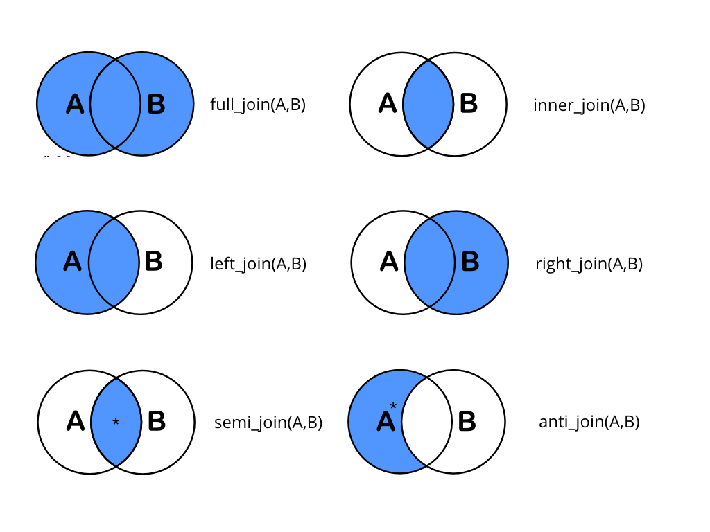
In practice, this is what it is doing:
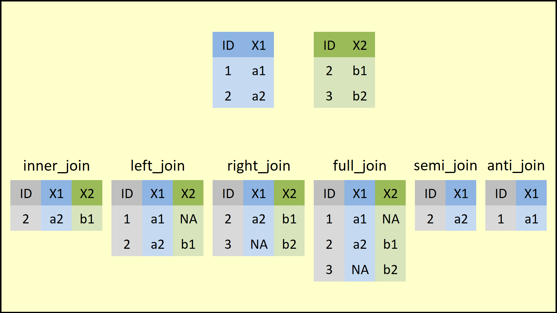
Joins are concerned with matching rows by a identifying key, deciding what to return (based on what we asked for) and returning all columns (semijoin and antijoin are exceptions to that).
The importance of ‘keys’
All joins rely on “keys” to match observations. A key is a unique identifier; it is usually a unique for each row. This can be a single column or the result of multiple columns. This information is used to match information in one table (or data frame) with another. The extent to which these keys match or do not match is the essence of a merge.
Let’s look at matches between “genotype”, “variety_trial”, and “metadata”.
The key between “metadata” and “variety_trial” is “trial”. There is exactly one row in the “metadata” file for each level of trial. The metadata file was designed to be like this. We did not need all those extra columns when it could be compressed into a smaller data set.
The file “genotype” is from a wholly different study. The extent of matches is considerably less complete than the matching between “variety_trial” and “metadata”.
Full join
All observations are returned, regardless if matched.
Let’s match “variety_trial” and “metadata”:
ex_fulljoin <- full_join(metadata, variety_trial, by = "trial")

dim(ex_fulljoin)
inner join
Returns only the rows with matching information. Non-matches are filtered out of the data set.
Let’s match “genotypes” and “variety_trial” (this will be big!).
How to check homany of these match (where the key is “variety” that matches “individual” in the object “genotypes”)?
base::intersect(variety_trial$variety, genotypes$individual)[1] "Jefferson" "UI Platinum" "LCS Star" "UI Stone" ex_innerjoin <- inner_join(variety_trial, genotypes, by = join_by("variety" == "individual"))Check results
dim(ex_innerjoin)[1] 76 10107sort(unique(ex_innerjoin$variety))[1] "Jefferson" "LCS Star" "UI Platinum" "UI Stone"
Practice Problems
Complete this expression:
test <- inner_join(genotypes, trial_1, by = join_by( ))Left join and right join
These preserves all the rows in one data set and matches to that dataset in the other. In the left join, it is the first data set (the one on the left) where all the rows are kep. In the right join, it’s the data set to the right that is full preserved.
Let’s compare the different when merging ‘trial_2’ with ‘metadata’.
Left join
ex_leftjoin_1 <- left_join(trial_2, metadata, by = "trial")
ex_leftjoin_2 <- left_join(metadata, trial_2, by = "trial")
Right join
#ex_rightjoin_1 <- right_join(metadata, trial_2, by = "trial")
ex_rightjoin_2 <- right_join(trial_2, metadata, by = "trial")
How are these 4 joins similar?
Answer
- ex_leftjoin_1 is the exact equivalent of ex_rightjoin_1, but the columns are in a different order.
- ex_leftjoin_2 is the exact equivalent of ex_rightjoin_2, but the columsn are in a different order.
Semi-join
One of my favorite joins! It does an inner join, but only return the columns for the first data set listed. It’s handy when you don’t want to generate gigantic objects.
Let’s revisit matching “genotypes” and “variety_trial” like in the inner_join() example above.
ex_semijoin <- semi_join(variety_trial, genotypes, by = join_by("variety" == "individual"))How do the dimensions of this object compare to the dimensions of ‘ex_innerjoin’?
Anti-join
This is similar to semi_join(). It will return all the rows that do not match, and only the columns from the first data set mentioned.
ex_antijoin <- anti_join(variety_trial, genotypes, by = join_by("variety" == "individual"))Do any of the variety names match?
table(ex_antijoin$variety %in% genotypes$individual)
FALSE
 1806
Note
dplyr can do complex joins.!
It can do some very flexible matching by numeric values, dates and other factors. More on this can be found in the documentation for join_by. This topic is complext and beyond the scope of this introductory workshop.
Practice Problems
- If not already imported, mport “genotypic_data_rotated.csv”, along with “trial_data.csv”, and “trial_metadata.csv”.
- Merge “genotypic_data_rotated.csv” and “trial_data.csv” that returns only varieties they have in common and columns from both data sets.
- Merge “genotypic_data_rotated.csv” and “trial_data.csv” that returns only varieties from “genotypic_data_rotated.csv” and the columns from “trial_data.csv”. Do the oppositie: varieties only in “trial_data.csv” and the columns from “genotypic_data_rotated.csv”.
- Do an anti-join between “genotypic_data_rotated.csv” and “trial_data.csv”.
- Join together all common observations between the 3 files (your choice on join).
Putting it all together
Although this lesson did not demonstrate the use of the pipe, %>%, it can be used with joins:
obj <- left_join(x, y) %>% right_join(z)The first join is a left join like any other. The second join presumes that the first argument is what was passed to it through the pipe. An equivalent:
temp <- left_join(x, y)
obj <-  right_join(temp, z)